Essentia Python tutorial
This is a hands-on tutorial for complete newcomers to Essentia. Essentia combines the power of computation speed of the main C++ code with the Python environment, making fast prototyping and scientific research very easy.
To follow this tutorial (and various Python examples we
provide)
interactively, we provide Jupyter Python
notebooks. They are located in the src/examples/python folder in
the source
code.
The notebook for this tutorial is essentia_python_tutorial.ipynb
(link).
If you are not familiar with Python notebooks, read how to use them
here.
You should have the NumPy package installed for computations with vectors and matrices in Python and Matplotlib for plotting. Other recommended packages for scientific computing not used in this tutorial but often used with Essentia are SciPy, scikit-learn, pandas, and seaborn for visualization.
The big strength of Essentia is its extensive collection of optimized and tested algorithms for audio processing and analysis, all conveniently available within the same library. You can parametrize and re-use these algorithms for specific use-cases and your custom analysis pipelines. For more details on the algorithms, see the algorithms overview and the complete algorithms reference.
Using Essentia in standard mode
There are two modes of using Essentia, standard and streaming, and in this section, we will focus on the standard mode. See next section for the streaming mode.
We will have a look at some basic functionality:
how to load an audio
how to perform some numerical operations such as FFT
how to plot results
how to output results to a file
Exploring the Python module
Let’s investigate a bit the Essentia package.
# first, we need to import our essentia module. It is aptly named 'essentia'!
import essentia

# there are two operating modes in essentia which (mostly) have the same algorithms
# they are accessible via two submodules:
import essentia.standard
import essentia.streaming

# let's have a look at what is in there
print(dir(essentia.standard))

# you can also do it by using autocompletion in Jupyter/IPython, typing "essentia.standard." and pressing Tab
['AfterMaxToBeforeMaxEnergyRatio', 'AllPass', 'AudioLoader', 'AudioOnsetsMarker', 'AudioWriter', 'AutoCorrelation', 'BFCC', 'BPF', 'BandPass', 'BandReject', 'BarkBands', 'BeatTrackerDegara', 'BeatTrackerMultiFeature', 'Beatogram', 'BeatsLoudness', 'BinaryOperator', 'BinaryOperatorStream', 'BpmHistogram', 'BpmHistogramDescriptors', 'BpmRubato', 'CartesianToPolar', 'CentralMoments', 'Centroid', 'ChordsDescriptors', 'ChordsDetection', 'ChordsDetectionBeats', 'Chromagram', 'Clipper', 'ConstantQ', 'Crest', 'CrossCorrelation', 'CubicSpline', 'DCRemoval', 'DCT', 'Danceability', 'Decrease', 'Derivative', 'DerivativeSFX', 'Dissonance', 'DistributionShape', 'Duration', 'DynamicComplexity', 'ERBBands', 'EasyLoader', 'EffectiveDuration', 'Energy', 'EnergyBand', 'EnergyBandRatio', 'Entropy', 'Envelope', 'EqloudLoader', 'EqualLoudness', 'Extractor', 'FFT', 'FFTC', 'FadeDetection', 'Flatness', 'FlatnessDB', 'FlatnessSFX', 'Flux', 'FrameCutter', 'FrameGenerator', 'FrameToReal', 'FreesoundExtractor', 'FrequencyBands', 'GFCC', 'GeometricMean', 'HFC', 'HPCP', 'HarmonicBpm', 'HarmonicMask', 'HarmonicModelAnal', 'HarmonicPeaks', 'HighPass', 'HighResolutionFeatures', 'HprModelAnal', 'HpsModelAnal', 'IDCT', 'IFFT', 'IIR', 'Inharmonicity', 'InstantPower', 'Intensity', 'Key', 'KeyExtractor', 'LPC', 'Larm', 'Leq', 'LevelExtractor', 'LogAttackTime', 'LoopBpmConfidence', 'LoopBpmEstimator', 'Loudness', 'LoudnessEBUR128', 'LoudnessVickers', 'LowLevelSpectralEqloudExtractor', 'LowLevelSpectralExtractor', 'LowPass', 'MFCC', 'Magnitude', 'MaxFilter', 'MaxMagFreq', 'MaxToTotal', 'Mean', 'Median', 'MelBands', 'MetadataReader', 'Meter', 'MinToTotal', 'MonoLoader', 'MonoMixer', 'MonoWriter', 'MovingAverage', 'MultiPitchKlapuri', 'MultiPitchMelodia', 'Multiplexer', 'MusicExtractor', 'NoiseAdder', 'NoveltyCurve', 'NoveltyCurveFixedBpmEstimator', 'OddToEvenHarmonicEnergyRatio', 'OnsetDetection', 'OnsetDetectionGlobal', 'OnsetRate', 'Onsets', 'OverlapAdd', 'PCA', 'Panning', 'PeakDetection', 'PercivalBpmEstimator', 'PercivalEnhanceHarmonics', 'PercivalEvaluatePulseTrains', 'PitchContourSegmentation', 'PitchContours', 'PitchContoursMelody', 'PitchContoursMonoMelody', 'PitchContoursMultiMelody', 'PitchFilter', 'PitchMelodia', 'PitchSalience', 'PitchSalienceFunction', 'PitchSalienceFunctionPeaks', 'PitchYin', 'PitchYinFFT', 'PolarToCartesian', 'PoolAggregator', 'PowerMean', 'PowerSpectrum', 'PredominantPitchMelodia', 'RMS', 'RawMoments', 'ReplayGain', 'Resample', 'ResampleFFT', 'RhythmDescriptors', 'RhythmExtractor', 'RhythmExtractor2013', 'RhythmTransform', 'RollOff', 'SBic', 'Scale', 'SilenceRate', 'SineModelAnal', 'SineModelSynth', 'SineSubtraction', 'SingleBeatLoudness', 'SingleGaussian', 'Slicer', 'SpectralCentroidTime', 'SpectralComplexity', 'SpectralContrast', 'SpectralPeaks', 'SpectralWhitening', 'Spectrum', 'SpectrumCQ', 'SpectrumToCent', 'Spline', 'SprModelAnal', 'SprModelSynth', 'SpsModelAnal', 'SpsModelSynth', 'StartStopSilence', 'StereoDemuxer', 'StereoMuxer', 'StereoTrimmer', 'StochasticModelAnal', 'StochasticModelSynth', 'StrongDecay', 'StrongPeak', 'SuperFluxExtractor', 'SuperFluxNovelty', 'SuperFluxPeaks', 'TCToTotal', 'TempoScaleBands', 'TempoTap', 'TempoTapDegara', 'TempoTapMaxAgreement', 'TempoTapTicks', 'TonalExtractor', 'TonicIndianArtMusic', 'TriangularBands', 'TriangularBarkBands', 'Trimmer', 'Tristimulus', 'TuningFrequency', 'TuningFrequencyExtractor', 'UnaryOperator', 'UnaryOperatorStream', 'Variance', 'Vibrato', 'WarpedAutoCorrelation', 'Windowing', 'YamlInput', 'YamlOutput', 'ZeroCrossingRate', '__builtins__', '__cached__', '__doc__', '__file__', '__loader__', '__name__', '__package__', '__spec__', '_c', '_create_essentia_class', '_create_python_algorithms', '_essentia', '_reloadAlgorithms', '_sys', 'algorithmInfo', 'algorithmNames', 'copy', 'essentia', 'iteritems']
This list contains all Essentia algorithms available in standard mode.
You can have an inline help for the algorithms you are interested in
using help command (you can also see it by typing MFCC in
Jupyter/IPython). You can also use our online algorithm
reference.
help(essentia.standard.MFCC)
Help on class Algo in module essentia.standard:

class Algo(Algorithm)
 |  MFCC
 |
 |
 |  Inputs:
 |
 |    [vector_real] spectrum - the audio spectrum
 |
 |
 |  Outputs:
 |
 |    [vector_real] bands - the energies in mel bands
 |    [vector_real] mfcc - the mel frequency cepstrum coefficients
 |
 |
 |  Parameters:
 |
 |    dctType:
 |      integer ∈ [2,3] (default = 2)
 |      the DCT type
 |
 |    highFrequencyBound:
 |      real ∈ (0,inf) (default = 11000)
 |      the upper bound of the frequency range [Hz]
 |
 |    inputSize:
 |      integer ∈ (1,inf) (default = 1025)
 |      the size of input spectrum
 |
 |    liftering:
 |      integer ∈ [0,inf) (default = 0)
 |      the liftering coefficient. Use '0' to bypass it
 |
 |    logType:
 |      string ∈ {natural,dbpow,dbamp,log} (default = "dbamp")
 |      logarithmic compression type. Use 'dbpow' if working with power and 'dbamp'
 |      if working with magnitudes
 |
 |    lowFrequencyBound:
 |      real ∈ [0,inf) (default = 0)
 |      the lower bound of the frequency range [Hz]
 |
 |    normalize:
 |      string ∈ {unit_sum,unit_max} (default = "unit_sum")
 |      'unit_max' makes the vertex of all the triangles equal to 1, 'unit_sum'
 |      makes the area of all the triangles equal to 1
 |
 |    numberBands:
 |      integer ∈ [1,inf) (default = 40)
 |      the number of mel-bands in the filter
 |
 |    numberCoefficients:
 |      integer ∈ [1,inf) (default = 13)
 |      the number of output mel coefficients
 |
 |    sampleRate:
 |      real ∈ (0,inf) (default = 44100)
 |      the sampling rate of the audio signal [Hz]
 |
 |    type:
 |      string ∈ {magnitude,power} (default = "power")
 |      use magnitude or power spectrum
 |
 |    warpingFormula:
 |      string ∈ {slaneyMel,htkMel} (default = "slaneyMel")
 |      The scale implementation type. use 'htkMel' to emulate its behaviour.
 |      Default slaneyMel.
 |
 |    weighting:
 |      string ∈ {warping,linear} (default = "warping")
 |      type of weighting function for determining triangle area
 |
 |
 |  Description:
 |
 |    This algorithm computes the mel-frequency cepstrum coefficients of a
 |    spectrum. As there is no standard implementation, the MFCC-FB40 is used by
 |    default:
 |      - filterbank of 40 bands from 0 to 11000Hz
 |      - take the log value of the spectrum energy in each mel band
 |      - DCT of the 40 bands down to 13 mel coefficients
 |    There is a paper describing various MFCC implementations [1].
 |
 |    The parameters of this algorithm can be configured in order to behave like
 |    HTK [3] as follows:
 |      - type = 'magnitude'
 |      - warpingFormula = 'htkMel'
 |      - weighting = 'linear'
 |      - highFrequencyBound = 8000
 |      - numberBands = 26
 |      - numberCoefficients = 13
 |      - normalize = 'unit_max'
 |      - dctType = 3
 |      - logType = 'log'
 |      - liftering = 22
 |
 |    In order to completely behave like HTK the audio signal has to be scaled by
 |    2^15 before the processing and if the Windowing and FrameCutter algorithms
 |    are used they should also be configured as follows.
 |
 |    FrameGenerator:
 |      - frameSize = 1102
 |      - hopSize = 441
 |      - startFromZero = True
 |      - validFrameThresholdRatio = 1
 |
 |    Windowing:
 |      - type = 'hamming'
 |      - size = 1102
 |      - zeroPadding = 946
 |      - normalized = False
 |
 |    This algorithm depends on the algorithms MelBands and DCT and therefore
 |    inherits their parameter restrictions. An exception is thrown if any of these
 |    restrictions are not met. The input "spectrum" is passed to the MelBands
 |    algorithm and thus imposes MelBands' input requirements. Exceptions are
 |    inherited by MelBands as well as by DCT.
 |
 |    IDCT can be used to compute smoothed Mel Bands. In order to do this:
 |     - compute MFCC
 |    - smoothedMelBands = 10^(IDCT(MFCC)/20)
 |
 |    Note: The second step assumes that 'logType' = 'dbamp' was used to compute
 |    MFCCs, otherwise that formula should be changed in order to be consistent.
 |
 |    References:
 |      [1] T. Ganchev, N. Fakotakis, and G. Kokkinakis, "Comparative evaluation
 |      of various MFCC implementations on the speaker verification task," in
 |      International Conference on Speach and Computer (SPECOM’05), 2005,
 |      vol. 1, pp. 191–194.
 |
 |      [2] Mel-frequency cepstrum - Wikipedia, the free encyclopedia,
 |      http://en.wikipedia.org/wiki/Mel_frequency_cepstral_coefficient
 |
 |      [3] Young, S. J., Evermann, G., Gales, M. J. F., Hain, T., Kershaw, D.,
 |      Liu, X., … Woodland, P. C. (2009). The HTK Book (for HTK Version 3.4).
 |      Construction, (July 2000), 384, https://doi.org/http://htk.eng.cam.ac.uk
 |
 |  Method resolution order:
 |      Algo
 |      Algorithm
 |      builtins.object
 |
 |  Methods defined here:
 |
 |  __call__(self, *args)
 |
 |  __init__(self, **kwargs)
 |
 |  __str__(self)
 |
 |  compute(self, *args)
 |
 |  configure(self, **kwargs)
 |
 |  ----------------------------------------------------------------------
 |  Data descriptors defined here:
 |
 |  __dict__
 |      dictionary for instance variables (if defined)
 |
 |  __weakref__
 |      list of weak references to the object (if defined)
 |
 |  ----------------------------------------------------------------------
 |  Data and other attributes defined here:
 |
 |  __struct__ = {'category': 'Spectral', 'description': 'This algorithm c...
 |
 |  ----------------------------------------------------------------------
 |  Methods inherited from Algorithm:
 |
 |  __compute__(...)
 |      compute the algorithm
 |
 |  __configure__(...)
 |      Configure the algorithm
 |
 |  __new__(*args, **kwargs) from builtins.type
 |      Create and return a new object.  See help(type) for accurate signature.
 |
 |  getDoc(...)
 |      Returns the doc string for the algorithm
 |
 |  getStruct(...)
 |      Returns the doc struct for the algorithm
 |
 |  inputNames(...)
 |      Returns the names of the inputs of the algorithm.
 |
 |  inputType(...)
 |      Returns the type of the input given by its name
 |
 |  name(...)
 |      Returns the name of the algorithm.
 |
 |  outputNames(...)
 |      Returns the names of the outputs of the algorithm.
 |
 |  paramType(...)
 |      Returns the type of the parameter given by its name
 |
 |  paramValue(...)
 |      Returns the value of the parameter or None if not yet configured
 |
 |  parameterNames(...)
 |      Returns the names of the parameters for this algorithm.
 |
 |  reset(...)
 |      Reset the algorithm to its initial state (if any).
Instantiating our first algorithm, loading some audio
Before you can use algorithms in Essentia, you first need to instantiate (create) them. When doing so, you can give them parameters which they may need to work properly, such as the filename of the audio file in the case of an audio loader.
Once you have instantiated an algorithm, nothing has happened yet, but your algorithm is ready to be used and works like a function, that is, you have to call it to make stuff happen (technically, it is a function object).
Essentia has a selection of audio loaders:
AudioLoader: the most generic one, returns the audio samples, sampling rate and number of channels, and some other related information
MonoLoader: returns audio, down-mixed and resampled to a given sampling rate
EasyLoader: a MonoLoader which can optionally trim start/end slices and rescale according to a ReplayGain value
EqloudLoader: an EasyLoader that applies an equal-loudness filtering to the audio
# we start by instantiating the audio loader:
loader = essentia.standard.MonoLoader(filename='../../../test/audio/recorded/dubstep.wav')

# and then we actually perform the loading:
audio = loader()
# This is how the audio we want to process sounds like
import IPython
IPython.display.Audio('../../../test/audio/recorded/dubstep.wav')
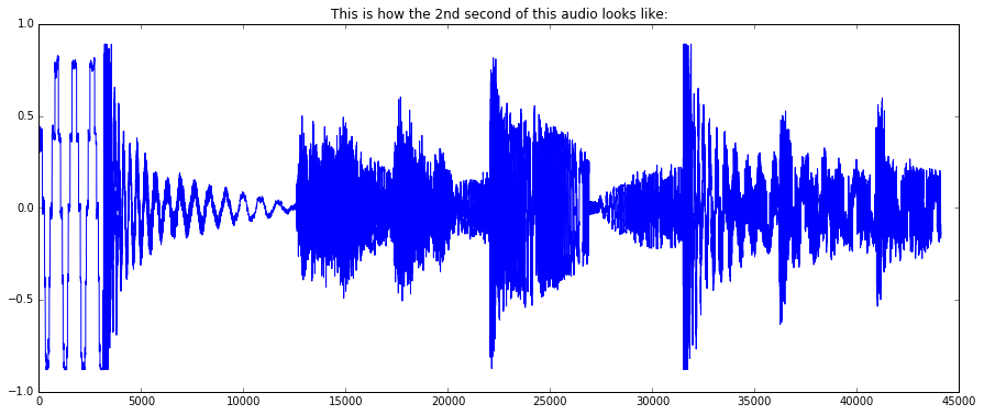
By default, the MonoLoader will output audio with 44100Hz sample rate downmixed to mono. To make sure that this actually worked, let’s plot a 1-second slice of audio, from t = 1 sec to t = 2 sec:
# pylab contains the plot() function, as well as figure, etc... (same names as Matlab)
from pylab import plot, show, figure, imshow
%matplotlib inline
import matplotlib.pyplot as plt
plt.rcParams['figure.figsize'] = (15, 6) # set plot sizes to something larger than default

plot(audio[1*44100:2*44100])
plt.title("This is how the 2nd second of this audio looks like:")
show()
Computing spectrum, mel bands energies, and MFCCs
So let’s say that we want to compute spectral energy in mel bands and the associated MFCCs for the frames in our audio.
We will need the following algorithms: Windowing, Spectrum, MFCC. For windowing, we’ll specify to use Hann window.
from essentia.standard import *
w = Windowing(type = 'hann')
spectrum = Spectrum()  # FFT() would return the complex FFT, here we just want the magnitude spectrum
mfcc = MFCC()
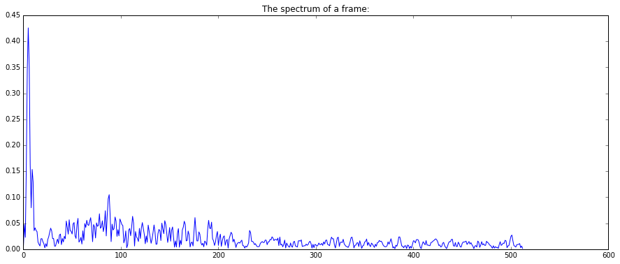
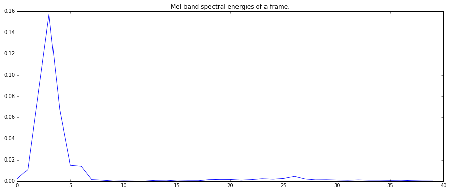
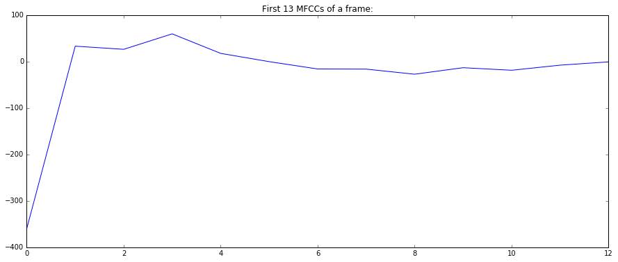
Once algorithms have been instantiated, they work like normal functions. Note that the MFCC algorithm returns two values: the band energies and the coefficients. Let’s compute and plot the spectrum, mel band energies, and MFCCs for a frame of audio:
frame = audio[6*44100 : 6*44100 + 1024]
spec = spectrum(w(frame))
mfcc_bands, mfcc_coeffs = mfcc(spec)

plot(spec)
plt.title("The spectrum of a frame:")
show()

plot(mfcc_bands)
plt.title("Mel band spectral energies of a frame:")
show()

plot(mfcc_coeffs)
plt.title("First 13 MFCCs of a frame:")
show()
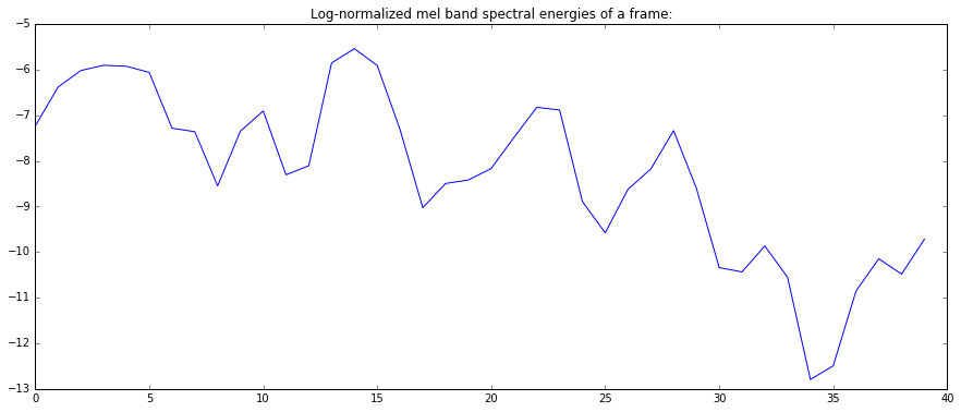
In the case of mel band energies, sometimes you may want to apply log normalization, which can be done using UnaryOperator. Using this algorithm we can do different types of normalization on vectors.
logNorm = UnaryOperator(type='log')
plot(logNorm(mfcc_bands))
plt.title("Log-normalized mel band spectral energies of a frame:")
show()
Computations on frames
Now let’s compute the mel band energies and MFCCs in all frames.
A typical Matlab-like way we would do it is by slicing the frames manually (the first frame starts at the moment 0, that is, with the first audio sample):
mfccs = []
melbands = []
frameSize = 1024
hopSize = 512

for fstart in range(0, len(audio)-frameSize, hopSize):
    frame = audio[fstart:fstart+frameSize]
    mfcc_bands, mfcc_coeffs = mfcc(spectrum(w(frame)))
    mfccs.append(mfcc_coeffs)
    melbands.append(mfcc_bands)
This is OK, but there is a much nicer way of computing frames in Essentia by using FrameGenerator, the FrameCutter algorithm wrapped into a Python generator:
mfccs = []
melbands = []
melbands_log = []

for frame in FrameGenerator(audio, frameSize=1024, hopSize=512, startFromZero=True):
    mfcc_bands, mfcc_coeffs = mfcc(spectrum(w(frame)))
    mfccs.append(mfcc_coeffs)
    melbands.append(mfcc_bands)
    melbands_log.append(logNorm(mfcc_bands))

# transpose to have it in a better shape
# we need to convert the list to an essentia.array first (== numpy.array of floats)
mfccs = essentia.array(mfccs).T
melbands = essentia.array(melbands).T
melbands_log = essentia.array(melbands_log).T

# and plot
imshow(melbands[:,:], aspect = 'auto', origin='lower', interpolation='none')
plt.title("Mel band spectral energies in frames")
show()

imshow(melbands_log[:,:], aspect = 'auto', origin='lower', interpolation='none')
plt.title("Log-normalized mel band spectral energies in frames")
show()

imshow(mfccs[1:,:], aspect='auto', origin='lower', interpolation='none')
plt.title("MFCCs in frames")
show()

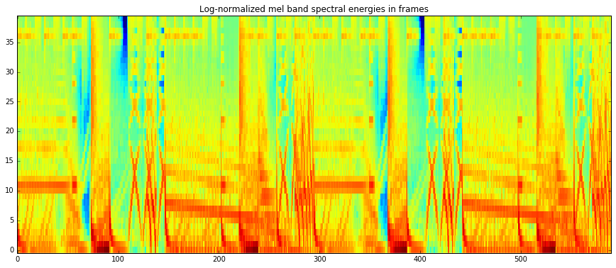

You can configure frame and hop size of the frame generator, and whether to start the first frame or to center it at zero position in time. For the complete list of available parameters see the documentation for the FrameCutter.
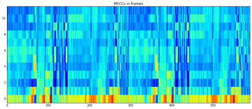
Note, that when plotting MFCCs, we ignored the first coefficient to disregard the power of the signal and only plot its spectral shape.
Storing results to Pool
A Pool is a container similar to a C++ map or Python dict which can
contain any type of values (easy in Python, not as much in C++…). Values
are stored in there using a name which represents the full path to these
values with dot (.) characters used as separators. You can think of
it as a directory tree, or as namespace(s) plus a local name.
Examples of valid names are: "bpm", "lowlevel.mfcc",
"highlevel.genre.rock.probability", etc…
Let’s redo the previous computations using a pool. The pool has the nice
advantage that the data you get out of it is already in an
essentia.array format (which is equal to numpy.array of floats), so
you can call transpose (.T) directly on it.
pool = essentia.Pool()

for frame in FrameGenerator(audio, frameSize = 1024, hopSize = 512, startFromZero=True):
    mfcc_bands, mfcc_coeffs = mfcc(spectrum(w(frame)))
    pool.add('lowlevel.mfcc', mfcc_coeffs)
    pool.add('lowlevel.mfcc_bands', mfcc_bands)
    pool.add('lowlevel.mfcc_bands_log', logNorm(mfcc_bands))

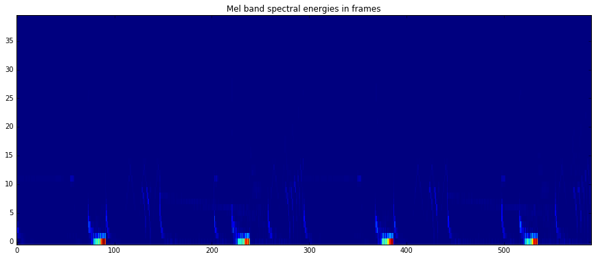
imshow(pool['lowlevel.mfcc_bands'].T, aspect = 'auto', origin='lower', interpolation='none')
plt.title("Mel band spectral energies in frames")
show()

imshow(pool['lowlevel.mfcc_bands_log'].T, aspect = 'auto', origin='lower', interpolation='none')
plt.title("Log-normalized mel band spectral energies in frames")
show()

imshow(pool['lowlevel.mfcc'].T[1:,:], aspect='auto', origin='lower', interpolation='none')
plt.title("MFCCs in frames")
show()

Aggregation and file output
As we are using Python, we could use its facilities for writing data to a file, but for the sake of this tutorial let’s do it using the YamlOutput algorithm, which writes a pool in a file using the YAML or JSON format.
output = YamlOutput(filename = 'mfcc.sig') # use "format = 'json'" for JSON output
output(pool)

# or as a one-liner:
YamlOutput(filename = 'mfcc.sig')(pool)
This can take a while as we actually write the MFCCs for all the frames, which can be quite heavy depending on the duration of your audio file.
Now let’s assume we do not want all the frames but only the mean and standard deviation of those frames. We can do this using the PoolAggregator algorithm on our pool with frame value to get a new pool with the aggregated descriptors (check the documentation for this algorithm to get an idea of other statistics it can compute):
# compute mean and variance of the frames
aggrPool = PoolAggregator(defaultStats = [ 'mean', 'stdev' ])(pool)

print('Original pool descriptor names:')
print(pool.descriptorNames())
print('')
print('Aggregated pool descriptor names:')
print(aggrPool.descriptorNames())
print('')

# and ouput those results in a file
YamlOutput(filename = 'mfccaggr.sig')(aggrPool)
Original pool descriptor names:
['lowlevel.mfcc', 'lowlevel.mfcc_bands', 'lowlevel.mfcc_bands_log']

Aggregated pool descriptor names:
['lowlevel.mfcc.mean', 'lowlevel.mfcc.stdev', 'lowlevel.mfcc_bands.mean', 'lowlevel.mfcc_bands.stdev', 'lowlevel.mfcc_bands_log.mean', 'lowlevel.mfcc_bands_log.stdev']
This is how the file with aggregated descriptors looks like:
!cat mfccaggr.sig
metadata:
    version:
        essentia: "2.1-dev"

lowlevel:
    mfcc:
        mean: [-548.465515137, 82.474647522, 23.9920558929, -3.92105984688, 9.37707233429, 0.0550536848605, 7.49981355667, 10.2677164078, 1.46692347527, 8.78695869446, -1.02505850792, 5.55843877792, -4.53198575974]
        stdev: [92.9804992676, 38.1891860962, 32.8111877441, 25.9349346161, 23.5974235535, 22.8900985718, 23.4571056366, 19.2605209351, 16.999912262, 17.3296813965, 18.9442825317, 18.8146419525, 16.8438053131]
    mfcc_bands:
        mean: [0.0430443286896, 0.0152214923874, 0.00659069558606, 0.00539278704673, 0.00387320877053, 0.00304042594507, 0.00343433767557, 0.00261196284555, 0.0023196185939, 0.00208778819069, 0.00157481990755, 0.00235125259496, 0.0010298260022, 0.000758393900469, 0.000447986851213, 0.000321425526636, 0.000237083833781, 0.000205824428122, 0.000197611472686, 0.000161219315487, 0.00013125318219, 0.000133611785714, 0.000161335541634, 0.000107279069198, 0.000109758009785, 0.000123509569676, 8.89756411198e-05, 6.59294382785e-05, 6.32342125755e-05, 5.04779345647e-05, 4.54452601844e-05, 4.45721161668e-05, 4.59850416519e-05, 3.38824975188e-05, 3.47260865965e-05, 4.02627483709e-05, 0.000151775820996, 5.23372145835e-05, 2.56655275734e-05, 2.47844927799e-05]
        stdev: [0.133796587586, 0.0390107147396, 0.0180664807558, 0.0187281165272, 0.0142051419243, 0.0091609954834, 0.0074247373268, 0.00607190933079, 0.00614743074402, 0.00666699418798, 0.0031948692631, 0.00523599097505, 0.00227958755568, 0.00226213759743, 0.00126964878291, 0.000707814877387, 0.000494667154271, 0.000490796519443, 0.000527630501892, 0.000423052668339, 0.000394845003029, 0.000347238150425, 0.000405938568292, 0.000299160223221, 0.000284110719804, 0.000375441013603, 0.000370208901586, 0.000277761428151, 0.000230042438488, 0.000162357377121, 0.000142114353366, 0.000132423578179, 0.00016263978614, 0.000110406210297, 0.000122218727483, 8.72409000294e-05, 0.000171674750163, 7.6599921158e-05, 4.17021510657e-05, 3.38126337738e-05]
    mfcc_bands_log:
        mean: [-6.24955272675, -6.57105016708, -7.34368038177, -7.92592859268, -8.36940193176, -8.14614963531, -7.9449005127, -8.2012386322, -8.46479320526, -8.75048446655, -8.32077884674, -8.22101211548, -8.66969203949, -9.37683773041, -9.66236972809, -9.83232212067, -9.74431324005, -9.8570098877, -10.0467433929, -10.6587133408, -10.9554595947, -10.5900297165, -10.5973072052, -10.9680480957, -11.1300811768, -11.0058526993, -11.3219165802, -11.7418317795, -11.9560842514, -11.8824300766, -11.7772083282, -11.8368644714, -11.8559484482, -12.1547746658, -11.830368042, -11.2242679596, -9.9259595871, -10.9285726547, -11.7089004517, -11.8566360474]
        stdev: [3.00452470779, 2.58188033104, 2.40453410149, 2.52647328377, 2.71612548828, 2.7103805542, 3.07109212875, 3.06873011589, 2.97640109062, 2.82126951218, 2.66976523399, 2.81773519516, 2.41420173645, 2.39151644707, 2.30262422562, 2.17882299423, 1.98866963387, 2.13317728043, 2.16317820549, 2.34757852554, 2.44092655182, 2.32866716385, 2.44926118851, 2.33606815338, 2.41704487801, 2.46625447273, 2.25014805794, 2.25670146942, 2.5483288765, 2.19981074333, 2.13154554367, 2.15053391457, 2.14865207672, 2.2223200798, 1.91899549961, 1.98338282108, 2.37033653259, 2.3670861721, 2.23138093948, 2.41583800316]
Summary and more examples
There is not much more to know for using Essentia in standard mode in Python, the basics are:
instantiate and configure algorithms
use them to compute some results
and that’s pretty much it!
You can find various Python examples in the src/examples/python
folder in the source
code,
for example:
computing spectral centroid (example_spectral_spectralcentroid.py)
onset detection (example_rhythm_onsetdetection.py)
predominant melody detection (example_pitch_predominantmelody.py and example_pitch_predominantmelody_by_steps.py)
Using Essentia in streaming mode
In this section, we will consider how to use Essentia in streaming mode.
The main difference between standard and streaming is that the standard mode is imperative while the streaming mode is declarative. That means that in standard mode, you tell exactly the computer what to do, whereas in the streaming mode, you “declare” what is needed to be done, and you let the computer do it itself. One big advantage of the streaming mode is that the memory consumption is greatly reduced, as you don’t need to load the entire audio in memory. Also, streaming mode allows reducing the amount of code which may be very significant for larger projects. Let’s have a look at it.
As usual, first import the essentia module:
import essentia
from essentia.streaming import *
Instantiate our algorithms:
loader = MonoLoader(filename = '../../../test/audio/recorded/dubstep.wav')
frameCutter = FrameCutter(frameSize = 1024, hopSize = 512)
w = Windowing(type = 'hann')
spec = Spectrum()
mfcc = MFCC()
In streaming, instead of calling algorithms like functions, we need to
connect their inputs and outputs. This is done using the >>
operator.
For example, the graph we want to connect looks like this:
----------      ------------      -----------      --------------      --------------
MonoLoader      FrameCutter       Windowing        Spectrum            MFCC
     audio ---> signal frame ---> frame frame ---> frame spectrum ---> spectrum bands ---> ???
                                                                                mfcc  ---> ???
----------      ------------      -----------      --------------      --------------
loader.audio >> frameCutter.signal
frameCutter.frame >> w.frame >> spec.frame
spec.spectrum >> mfcc.spectrum
<essentia.streaming._StreamConnector at 0x7f11817e3940>
When building a network, all inputs need to be connected, no matter what, otherwise the network cannot be started and we get an error message:
essentia.run(loader)
---------------------------------------------------------------------------

RuntimeError                              Traceback (most recent call last)

<ipython-input-17-5a68facf7b1d> in <module>()
----> 1 essentia.run(loader)


/usr/local/lib/python3.5/dist-packages/essentia/__init__.py in run(gen)
    146     if isinstance(gen, VectorInput) and not list(gen.connections.values())[0]:
    147         raise EssentiaError('VectorInput is not connected to anything...')
--> 148     return _essentia.run(gen)
    149
    150 log.debug(EPython, 'Successfully imported essentia python module (log fully available and synchronized with the C++ one)')


RuntimeError: MFCC::bands is not connected to any sink...
In our case, the outputs of the MFCC algorithm were not connected anywhere. Let’s store mfcc values in the pool and ignore bands values.
----------      ------------      -----------      --------------      --------------
MonoLoader      FrameCutter       Windowing        Spectrum            MFCC
     audio ---> signal frame ---> frame frame ---> frame spectrum ---> spectrum bands ---> NOWHERE
                                                                                mfcc  ---> Pool: lowlevel.mfcc
----------      ------------      -----------      --------------      --------------
pool = essentia.Pool()

mfcc.bands >> None
mfcc.mfcc >> (pool, 'lowlevel.mfcc')

essentia.run(loader)

print('Pool contains %d frames of MFCCs' % len(pool['lowlevel.mfcc']))
Pool contains 592 frames of MFCCs
Let’s try writing directly to a text file instead of a pool and yaml files
We first need to disconnect the old connection to the pool to avoid putting the same data in there again.
mfcc.mfcc.disconnect((pool, 'lowlevel.mfcc'))
We create a FileOutput and connect it. It is a special connection that has no input because it can actually take any type of input (the other algorithms will complain if you try to connect an output to an input of a different type).
fileout = FileOutput(filename = 'mfccframes.txt')
mfcc.mfcc >> fileout
<essentia.streaming._create_streaming_algo.<locals>.StreamingAlgo at 0x7f11815d5d38>
Reset the network otherwise the loader in particular will not do anything useful, and rerun the network
essentia.reset(loader)
essentia.run(loader)
This is the resulting file (the first 10 lines correspond to the first 10 frames):
!head mfccframes.txt -n 10
[-430.671, 87.7917, -10.1204, -50.172, -17.9259, -36.4849, -17.5709, -5.72504, -16.6404, 8.64975, -7.41039, 5.7051, 7.18055]
[-490.824, 101.549, 68.3375, 10.5324, 9.86464, -21.2722, -12.467, -11.8749, -24.2667, -8.02748, -26.5459, -25.3716, -31.5997]
[-515.915, 90.4185, 54.5073, 25.2965, 18.2453, 1.56025, 10.0262, 21.2547, 2.83289, 7.16083, -25.8393, -22.4263, -29.8229]
[-526.075, 76.321, 33.0371, 15.6267, 16.1482, 1.94901, 26.5443, 40.805, 20.866, 20.7323, -16.962, -23.6936, -39.9292]
[-530.409, 62.8531, 17.8901, 17.2312, 19.4443, 6.44692, 35.9218, 37.0124, 9.91326, 30.9235, -10.691, -12.6595, -30.0003]
[-532.03, 66.9765, 15.174, 4.41039, 6.51187, 18.4618, 41.4819, 30.0178, 13.5438, 19.5735, -19.7553, -2.62841, -12.9201]
[-523.106, 85.9242, 15.2094, 11.4087, 9.95426, 19.4773, 20.8585, 27.0054, 19.3617, 19.016, -13.5927, -3.25358, -11.339]
[-532.996, 90.4333, 13.19, 8.79797, 20.2316, 15.791, 23.7306, 34.2449, 11.5618, 20.3763, -18.6916, -10.9794, -20.2573]
[-539.285, 74.0864, 20.9641, 18.1156, 11.1981, 6.7221, 25.9186, 38.2328, 8.60174, 16.578, -22.699, -19.8375, -27.6012]
[-512.555, 60.0025, 25.2892, 3.13255, 18.0855, -2.79686, 22.4047, 25.8552, 6.91858, 11.1513, -10.3943, -17.6128, -8.85415]
Examples
extracting key by steps (example_key_by_steps_streaming.py)