Essentia Python examples
This Jupyter notebook demonstrates various typical examples of using Essentia in Python.
Computing features with MusicExtractor
MusicExtractor is a multi-purpose algorithm for feature extraction from files (see the complete list of computed features here). It combines many algorithms and is also used inside the Essentia’s command-line Music Extractor. For any given input filename, all computed features are stored in two output Pools which you can access for your needs or store to a file. One of the pools contains raw frames data, while another one contains aggregated statistics across frames.
# This is how the audio we want to process sounds like
import IPython
IPython.display.Audio('../../../test/audio/recorded/dubstep.flac')
import essentia
import essentia.standard as es
# Compute all features, aggregate only 'mean' and 'stdev' statistics for all low-level, rhythm and tonal frame features
features, features_frames = es.MusicExtractor(lowlevelStats=['mean', 'stdev'],
rhythmStats=['mean', 'stdev'],
tonalStats=['mean', 'stdev'])('../../../test/audio/recorded/dubstep.flac')
# See all feature names in the pool in a sorted order
print(sorted(features.descriptorNames()))
['lowlevel.average_loudness', 'lowlevel.barkbands.mean', 'lowlevel.barkbands.stdev', 'lowlevel.barkbands_crest.mean', 'lowlevel.barkbands_crest.stdev', 'lowlevel.barkbands_flatness_db.mean', 'lowlevel.barkbands_flatness_db.stdev', 'lowlevel.barkbands_kurtosis.mean', 'lowlevel.barkbands_kurtosis.stdev', 'lowlevel.barkbands_skewness.mean', 'lowlevel.barkbands_skewness.stdev', 'lowlevel.barkbands_spread.mean', 'lowlevel.barkbands_spread.stdev', 'lowlevel.dissonance.mean', 'lowlevel.dissonance.stdev', 'lowlevel.dynamic_complexity', 'lowlevel.erbbands.mean', 'lowlevel.erbbands.stdev', 'lowlevel.erbbands_crest.mean', 'lowlevel.erbbands_crest.stdev', 'lowlevel.erbbands_flatness_db.mean', 'lowlevel.erbbands_flatness_db.stdev', 'lowlevel.erbbands_kurtosis.mean', 'lowlevel.erbbands_kurtosis.stdev', 'lowlevel.erbbands_skewness.mean', 'lowlevel.erbbands_skewness.stdev', 'lowlevel.erbbands_spread.mean', 'lowlevel.erbbands_spread.stdev', 'lowlevel.gfcc.cov', 'lowlevel.gfcc.icov', 'lowlevel.gfcc.mean', 'lowlevel.hfc.mean', 'lowlevel.hfc.stdev', 'lowlevel.loudness_ebu128.integrated', 'lowlevel.loudness_ebu128.loudness_range', 'lowlevel.loudness_ebu128.momentary.mean', 'lowlevel.loudness_ebu128.momentary.stdev', 'lowlevel.loudness_ebu128.short_term.mean', 'lowlevel.loudness_ebu128.short_term.stdev', 'lowlevel.melbands.mean', 'lowlevel.melbands.stdev', 'lowlevel.melbands128.mean', 'lowlevel.melbands128.stdev', 'lowlevel.melbands_crest.mean', 'lowlevel.melbands_crest.stdev', 'lowlevel.melbands_flatness_db.mean', 'lowlevel.melbands_flatness_db.stdev', 'lowlevel.melbands_kurtosis.mean', 'lowlevel.melbands_kurtosis.stdev', 'lowlevel.melbands_skewness.mean', 'lowlevel.melbands_skewness.stdev', 'lowlevel.melbands_spread.mean', 'lowlevel.melbands_spread.stdev', 'lowlevel.mfcc.cov', 'lowlevel.mfcc.icov', 'lowlevel.mfcc.mean', 'lowlevel.pitch_salience.mean', 'lowlevel.pitch_salience.stdev', 'lowlevel.silence_rate_20dB.mean', 'lowlevel.silence_rate_20dB.stdev', 'lowlevel.silence_rate_30dB.mean', 'lowlevel.silence_rate_30dB.stdev', 'lowlevel.silence_rate_60dB.mean', 'lowlevel.silence_rate_60dB.stdev', 'lowlevel.spectral_centroid.mean', 'lowlevel.spectral_centroid.stdev', 'lowlevel.spectral_complexity.mean', 'lowlevel.spectral_complexity.stdev', 'lowlevel.spectral_contrast_coeffs.mean', 'lowlevel.spectral_contrast_coeffs.stdev', 'lowlevel.spectral_contrast_valleys.mean', 'lowlevel.spectral_contrast_valleys.stdev', 'lowlevel.spectral_decrease.mean', 'lowlevel.spectral_decrease.stdev', 'lowlevel.spectral_energy.mean', 'lowlevel.spectral_energy.stdev', 'lowlevel.spectral_energyband_high.mean', 'lowlevel.spectral_energyband_high.stdev', 'lowlevel.spectral_energyband_low.mean', 'lowlevel.spectral_energyband_low.stdev', 'lowlevel.spectral_energyband_middle_high.mean', 'lowlevel.spectral_energyband_middle_high.stdev', 'lowlevel.spectral_energyband_middle_low.mean', 'lowlevel.spectral_energyband_middle_low.stdev', 'lowlevel.spectral_entropy.mean', 'lowlevel.spectral_entropy.stdev', 'lowlevel.spectral_flux.mean', 'lowlevel.spectral_flux.stdev', 'lowlevel.spectral_kurtosis.mean', 'lowlevel.spectral_kurtosis.stdev', 'lowlevel.spectral_rms.mean', 'lowlevel.spectral_rms.stdev', 'lowlevel.spectral_rolloff.mean', 'lowlevel.spectral_rolloff.stdev', 'lowlevel.spectral_skewness.mean', 'lowlevel.spectral_skewness.stdev', 'lowlevel.spectral_spread.mean', 'lowlevel.spectral_spread.stdev', 'lowlevel.spectral_strongpeak.mean', 'lowlevel.spectral_strongpeak.stdev', 'lowlevel.zerocrossingrate.mean', 'lowlevel.zerocrossingrate.stdev', 'metadata.audio_properties.analysis.downmix', 'metadata.audio_properties.analysis.equal_loudness', 'metadata.audio_properties.analysis.length', 'metadata.audio_properties.analysis.sample_rate', 'metadata.audio_properties.analysis.start_time', 'metadata.audio_properties.bit_rate', 'metadata.audio_properties.codec', 'metadata.audio_properties.length', 'metadata.audio_properties.lossless', 'metadata.audio_properties.md5_encoded', 'metadata.audio_properties.number_channels', 'metadata.audio_properties.replay_gain', 'metadata.audio_properties.sample_rate', 'metadata.tags.file_name', 'metadata.version.essentia', 'metadata.version.essentia_git_sha', 'metadata.version.extractor', 'rhythm.beats_count', 'rhythm.beats_loudness.mean', 'rhythm.beats_loudness.stdev', 'rhythm.beats_loudness_band_ratio.mean', 'rhythm.beats_loudness_band_ratio.stdev', 'rhythm.beats_position', 'rhythm.bpm', 'rhythm.bpm_histogram', 'rhythm.bpm_histogram_first_peak_bpm', 'rhythm.bpm_histogram_first_peak_weight', 'rhythm.bpm_histogram_second_peak_bpm', 'rhythm.bpm_histogram_second_peak_spread', 'rhythm.bpm_histogram_second_peak_weight', 'rhythm.danceability', 'rhythm.onset_rate', 'tonal.chords_changes_rate', 'tonal.chords_histogram', 'tonal.chords_key', 'tonal.chords_number_rate', 'tonal.chords_scale', 'tonal.chords_strength.mean', 'tonal.chords_strength.stdev', 'tonal.hpcp.mean', 'tonal.hpcp.stdev', 'tonal.hpcp_crest.mean', 'tonal.hpcp_crest.stdev', 'tonal.hpcp_entropy.mean', 'tonal.hpcp_entropy.stdev', 'tonal.key_edma.key', 'tonal.key_edma.scale', 'tonal.key_edma.strength', 'tonal.key_krumhansl.key', 'tonal.key_krumhansl.scale', 'tonal.key_krumhansl.strength', 'tonal.key_temperley.key', 'tonal.key_temperley.scale', 'tonal.key_temperley.strength', 'tonal.thpcp', 'tonal.tuning_diatonic_strength', 'tonal.tuning_equal_tempered_deviation', 'tonal.tuning_frequency', 'tonal.tuning_nontempered_energy_ratio']
You can then access particular values in the pools:
print("Filename:", features['metadata.tags.file_name'])
print("-"*80)
print("Replay gain:", features['metadata.audio_properties.replay_gain'])
print("EBU128 integrated loudness:", features['lowlevel.loudness_ebu128.integrated'])
print("EBU128 loudness range:", features['lowlevel.loudness_ebu128.loudness_range'])
print("-"*80)
print("MFCC mean:", features['lowlevel.mfcc.mean'])
print("-"*80)
print("BPM:", features['rhythm.bpm'])
print("Beat positions (sec.)", features['rhythm.beats_position'])
print("-"*80)
print("Key/scale estimation (using a profile specifically suited for electronic music):",
features['tonal.key_edma.key'], features['tonal.key_edma.scale'])
Filename: dubstep.flac
--------------------------------------------------------------------------------
Replay gain: -13.708175659179688
EBU128 integrated loudness: -10.151906967163086
EBU128 loudness range: 0.6067428588867188
--------------------------------------------------------------------------------
MFCC mean: [-670.34771729 84.01703644 24.20178986 -4.55752945 8.39075661
-1.40908575 6.48751211 9.55739212 1.58020043 9.26296902
-0.74807823 5.43698931 -4.19750071]
--------------------------------------------------------------------------------
BPM: 139.98114013671875
Beat positions (sec.) [ 0.42956915 0.85913831 1.30031741 1.71827662 2.14784575 2.57741499
2.9953742 3.42494321 3.86612248 4.29569149 4.72526073 5.15482998
5.58439922 6.01396799 6.4319272 ]
--------------------------------------------------------------------------------
Key/scale estimation (using a profile specifically suited for electronic music): G# minor
Beat detection and BPM histogram
In this example we are going to look at how to perform beat tracking using RhythmExtractor2013, mark the extractred beats on the audio using the AudioOnsetsMarker algorithm and write those to file using MonoWriter.
from essentia.standard import *
# Loading audio file
audio = MonoLoader(filename='../../../test/audio/recorded/dubstep.flac')()
# Compute beat positions and BPM
rhythm_extractor = RhythmExtractor2013(method="multifeature")
bpm, beats, beats_confidence, _, beats_intervals = rhythm_extractor(audio)
print("BPM:", bpm)
print("Beat positions (sec.):", beats)
print("Beat estimation confidence:", beats_confidence)
# Mark beat positions on the audio and write it to a file
# Let's use beeps instead of white noise to mark them, as it's more distinctive
marker = AudioOnsetsMarker(onsets=beats, type='beep')
marked_audio = marker(audio)
MonoWriter(filename='audio/dubstep_beats.flac')(marked_audio)
BPM: 139.98114013671875
Beat positions (sec.): [ 0.42956915 0.85913831 1.30031741 1.71827662 2.14784575 2.57741499
2.9953742 3.42494321 3.86612248 4.29569149 4.72526073 5.15482998
5.58439922 6.01396799 6.4319272 ]
Beat estimation confidence: 3.9443612098693848
We can now listen to the resulting audio with beats marked by beeps. We can also visualize beat estimations.
import IPython
IPython.display.Audio('audio/dubstep_beats.flac')
from pylab import plot, show, figure, imshow
%matplotlib inline
import matplotlib.pyplot as plt
plt.rcParams['figure.figsize'] = (15, 6) # set plot sizes to something larger than default
plot(audio)
for beat in beats:
plt.axvline(x=beat*44100, color='red')
plt.title("Audio waveform and the estimated beat positions")
<matplotlib.text.Text at 0x7fef3902d3c8>
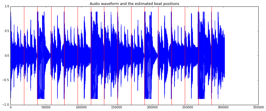
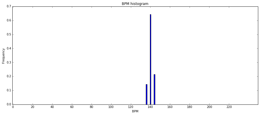
The BPM value output by RhythmExtactor2013 is the average of all BPM estimates done for each interval between two consecutive beats. Alternatively, we could analyze the distribution of all those intervals using BpmHistogramDescriptors. This would especially make sense for music with a varying rhythm (which is not the case in our example, but anyways…).
peak1_bpm, peak1_weight, peak1_spread, peak2_bpm, peak2_weight, peak2_spread, histogram = BpmHistogramDescriptors()(beats_intervals)
print("Overall BPM (estimated before): %0.1f" % bpm)
print("First histogram peak: %0.1f bpm" % peak1_bpm)
print("Second histogram peak: %0.1f bpm" % peak2_bpm)
fig, ax = plt.subplots()
ax.bar(range(len(histogram)), histogram, width=1)
ax.set_xlabel('BPM')
ax.set_ylabel('Frequency')
plt.title("BPM histogram")
ax.set_xticks([20 * x + 0.5 for x in range(int(len(histogram) / 20))])
ax.set_xticklabels([str(20 * x) for x in range(int(len(histogram) / 20))])
plt.show()
Overall BPM (estimated before): 140.0
First histogram peak: 140.0 bpm
Second histogram peak: 0.0 bpm
Onset detection
In this example we are going to look at how to perform onset detection and mark onsets on the audio using the AudioOnsetsMarker algorithm.
Onset detection consists of two main phases: - Compute an onset detection function, which is a function describing the evolution of some parameters, which might be representative of whether we might find an onset or not - Decide onset locations in the signal based on a number of these detection functions
The OnsetDetection algorithm estimates various onset detection functions for an audio frame given its spectrum. Onsets detects onsets given a matrix with values of onset detection functions in each frame.
It might be hard to hear the sound of hihats as it gets masked by the onset beeps in the mono signal. As an alternative, we can store both the original sound and the beeps in a stereo signal putting them separately into left and right channels using StereoMuxer and AudioWriter.
# Loading audio file
audio = MonoLoader(filename='../../../test/audio/recorded/hiphop.mp3')()
# Phase 1: compute the onset detection function
# The OnsetDetection algorithm provides various onset detection functions. Let's use two of them.
od1 = OnsetDetection(method='hfc')
od2 = OnsetDetection(method='complex')
# Let's also get the other algorithms we will need, and a pool to store the results
w = Windowing(type = 'hann')
fft = FFT() # this gives us a complex FFT
c2p = CartesianToPolar() # and this turns it into a pair (magnitude, phase)
pool = essentia.Pool()
# Computing onset detection functions.
for frame in FrameGenerator(audio, frameSize = 1024, hopSize = 512):
mag, phase, = c2p(fft(w(frame)))
pool.add('features.hfc', od1(mag, phase))
pool.add('features.complex', od2(mag, phase))
# Phase 2: compute the actual onsets locations
onsets = Onsets()
onsets_hfc = onsets(# this algo expects a matrix, not a vector
essentia.array([ pool['features.hfc'] ]),
# you need to specify weights, but as there is only a single
# function, it doesn't actually matter which weight you give it
[ 1 ])
onsets_complex = onsets(essentia.array([ pool['features.complex'] ]), [ 1 ])
# Mark onsets on the audio, which we'll write back to disk
# We use beeps instead of white noise and stereo signal as it's more distinctive
silence = [0.] * len(audio)
beeps_hfc = AudioOnsetsMarker(onsets=onsets_hfc, type='beep')(silence)
AudioWriter(filename='audio/hiphop_onsets_hfc_stereo.mp3', format='mp3')(StereoMuxer()(audio, beeps_hfc))
beeps_complex = AudioOnsetsMarker(onsets=onsets_complex, type='beep')(silence)
AudioWriter(filename='audio/hiphop_onsets_complex_stereo.mp3', format='mp3')(StereoMuxer()(audio, beeps_complex))
We can now go listen to the resulting audio files to see which onset detection function works better.
IPython.display.Audio('../../../test/audio/recorded/hiphop.mp3')
IPython.display.Audio('audio/hiphop_onsets_hfc_stereo.mp3')
IPython.display.Audio('audio/hiphop_onsets_complex_stereo.mp3')
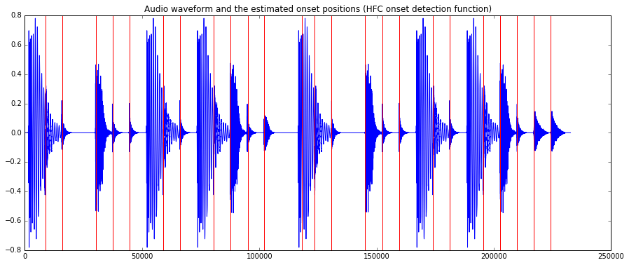
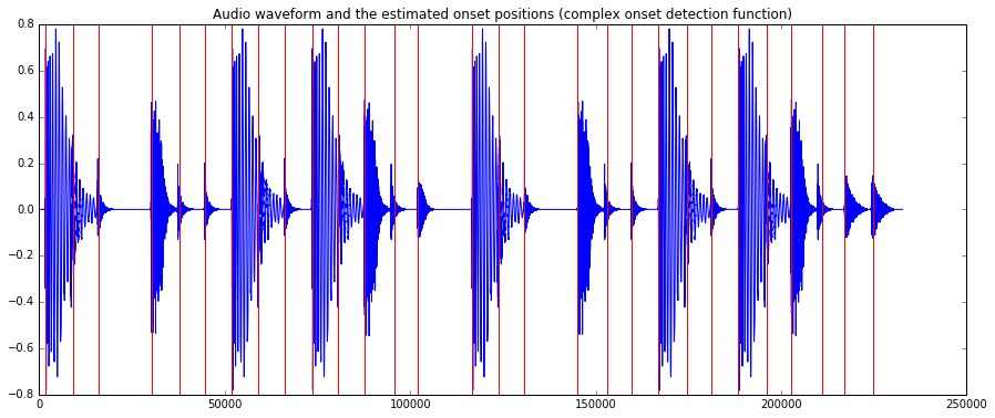
Finally, inspecting the plots with onsets marked by vertical lines, we can easily see how the HFC method picks up the highhats, which the complex method also detects the kicks.
plot(audio)
for onset in onsets_hfc:
plt.axvline(x=onset*44100, color='red')
plt.title("Audio waveform and the estimated onset positions (HFC onset detection function)")
plt.show()
plot(audio)
for onset in onsets_complex:
plt.axvline(x=onset*44100, color='red')
plt.title("Audio waveform and the estimated onset positions (complex onset detection function)")
<matplotlib.text.Text at 0x7fef38c85278>
Melody detection
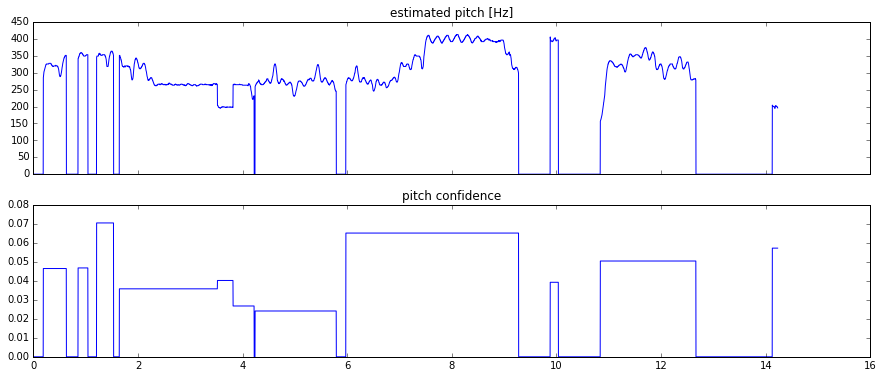
In this example we will analyse the pitch contour of the predominant melody in an audio recording using the PredominantPitchMelodia algorithm. This algorithm outputs a time series (sequence of values) with the instantaneous pitch value (in Hertz) of the perceived melody. It can be used with both monophonic and polyphonic signals.
import numpy
# Load audio file; it is recommended to apply equal-loudness filter for PredominantPitchMelodia
loader = EqloudLoader(filename='../python/musicbricks-tutorials/flamenco.wav', sampleRate=44100)
audio = loader()
print("Duration of the audio sample [sec]:")
print(len(audio)/44100.0)
# Extract the pitch curve
# PitchMelodia takes the entire audio signal as input (no frame-wise processing is required)
pitch_extractor = PredominantPitchMelodia(frameSize=2048, hopSize=128)
pitch_values, pitch_confidence = pitch_extractor(audio)
# Pitch is estimated on frames. Compute frame time positions
pitch_times = numpy.linspace(0.0,len(audio)/44100.0,len(pitch_values) )
# Plot the estimated pitch contour and confidence over time
f, axarr = plt.subplots(2, sharex=True)
axarr[0].plot(pitch_times, pitch_values)
axarr[0].set_title('estimated pitch [Hz]')
axarr[1].plot(pitch_times, pitch_confidence)
axarr[1].set_title('pitch confidence')
plt.show()
Duration of the audio sample [sec]:
14.22859410430839
Let’s listen to the estimated pitch and compare it to the original audio.
# TODO
Tonality analysis (HPCP, key and scale)
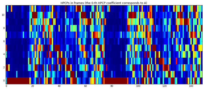
In this example we will analyze tonality of a music track. We will analyze the spectrum of an audio signal, find out its spectral peaks using SpectralPeak and then estimate the harmonic pitch class profile using the HPCP algorithm. Finally, we will estimate key and scale of the track based on its HPCP value using the Key algorithm.
In this particular case, it is easier to write the code in streaming mode as it is much simpler.
import essentia.streaming as ess
# Initialize algorithms we will use
loader = ess.MonoLoader(filename='../../../test/audio/recorded/dubstep.flac')
framecutter = ess.FrameCutter(frameSize=4096, hopSize=2048, silentFrames='noise')
windowing = ess.Windowing(type='blackmanharris62')
spectrum = ess.Spectrum()
spectralpeaks = ess.SpectralPeaks(orderBy='magnitude',
magnitudeThreshold=0.00001,
minFrequency=20,
maxFrequency=3500,
maxPeaks=60)
# Use default HPCP parameters for plots, however we will need higher resolution
# and custom parameters for better Key estimation
hpcp = ess.HPCP()
hpcp_key = ess.HPCP(size=36, # we will need higher resolution for Key estimation
referenceFrequency=440, # assume tuning frequency is 44100.
bandPreset=False,
minFrequency=20,
maxFrequency=3500,
weightType='cosine',
nonLinear=False,
windowSize=1.)
key = ess.Key(profileType='edma', # Use profile for electronic music
numHarmonics=4,
pcpSize=36,
slope=0.6,
usePolyphony=True,
useThreeChords=True)
# Use pool to store data
pool = essentia.Pool()
# Connect streaming algorithms
loader.audio >> framecutter.signal
framecutter.frame >> windowing.frame >> spectrum.frame
spectrum.spectrum >> spectralpeaks.spectrum
spectralpeaks.magnitudes >> hpcp.magnitudes
spectralpeaks.frequencies >> hpcp.frequencies
spectralpeaks.magnitudes >> hpcp_key.magnitudes
spectralpeaks.frequencies >> hpcp_key.frequencies
hpcp_key.hpcp >> key.pcp
hpcp.hpcp >> (pool, 'tonal.hpcp')
key.key >> (pool, 'tonal.key_key')
key.scale >> (pool, 'tonal.key_scale')
key.strength >> (pool, 'tonal.key_strength')
# Run streaming network
essentia.run(loader)
# Plot HPCP
imshow(pool['tonal.hpcp'].T, aspect='auto', origin='lower', interpolation='none')
plt.title("HPCPs in frames (the 0-th HPCP coefficient corresponds to A)")
show()
print("Estimated key and scale:", pool['tonal.key_key'] + " " + pool['tonal.key_scale'])
Estimated key and scale: A minor
Fingerprinting
Using Chromaprint wrapper to identify audio with AcousticID
Chromaprint is a fingerprinting algorithm based on chroma features. AcoustID is a web service that relies on chromaprints in order to identify tracks from the MusicBrainz database.
Queries to AcousticID requires a client key, the song duration and the fingerprint. Additionally, a query can ask for extra metadata from the MusicBrainz database using the field meta (https://acoustid.org/webservice).
Essentia provides a wrapper algorithm, Chromaprinter, for computing fingerprints with the Chromaprint library. In the standard mode, a fingerprint is computed for the whole audio duration and it can be used to generate a query as in the example below:
# the specified file is not provided with this notebook, try using your own music instead
audio = es.MonoLoader(filename='Desakato-Tiempo de cobardes.mp3', sampleRate=44100)()
fingerprint = es.Chromaprinter()(audio)
client = 'hGU_Gmo7vAY' # This is not a valid key. Use your key.
duration = len(audio) / 44100.
# Composing a query asking for the fields: recordings, releasegroups and compress.
query = 'http://api.acoustid.org/v2/lookup?client=%s&meta=recordings+releasegroups+compress&duration=%i&fingerprint=%s' \
%(client, duration, fingerprint)
from six.moves import urllib
page = urllib.request.urlopen(query)
print(page.read())
{"status": "ok", "results": [{"recordings": [{"artists": [{"id": "b02d0e59-b9c2-4009-9ebd-bfac7ffa0ca3", "name": "Desakato"}], "duration": 129, "releasegroups": [{"type": "Album", "id": "a38dc1ea-74fc-44c2-a31c-783810ba1568", "title": "La Teoru00eda del Fuego"}], "title": "Tiempo de cobardes", "id": "9b91e561-a9bf-415a-957b-33e6130aba76"}], "score": 0.937038, "id": "23495e47-d670-4e86-bd08-b1b24a84f7c7"}]}
Chromaprints can also be computed real-time using the streaming mode. In
this case, a fingerprint is computed each analysisTime seconds. In
order to offer the same behaviour seen in the standard mode, the
fingerprint can be internally stored until the end of the signal using
the concatenate flag (True by default). In this case, only one
chromaprint is returned when the audio stream ends.
loader = ess.MonoLoader(filename = 'Music/Desakato-La_Teoria_del_Fuego/01. Desakato-Tiempo de cobardes.mp3')
fps = ess.Chromaprinter(analysisTime=20, concatenate=True)
pool = ess.essentia.Pool()
# Conecting the algorithms
loader.audio >> fps.signal
fps.fingerprint >> (pool, 'chromaprint')
ess.essentia.run(loader)
fp = pool['chromaprint'][0]
In order to make the fingerprints more handy, they are compressed as
char arrays. We can make use of the decode_fingerprint functionality
by the pyacoustid package in
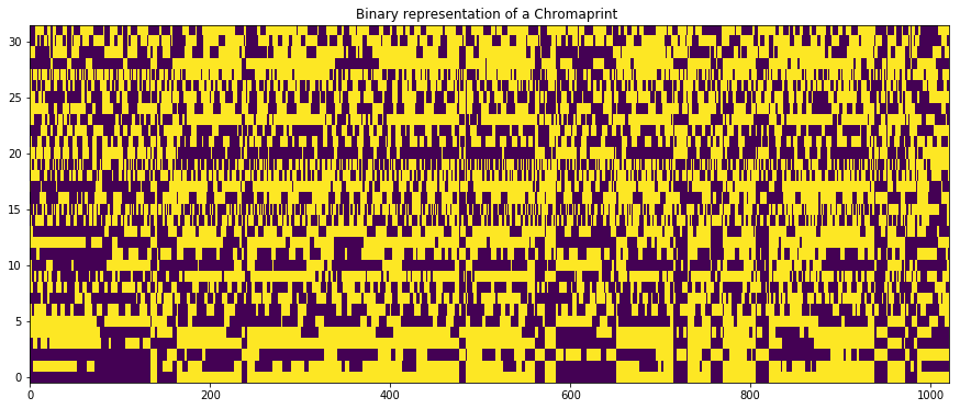
order to get the integer representation of the Chromaprint and visualize
it.
import acoustid as ai
fp_int = ai.chromaprint.decode_fingerprint(fp)[0]
fb_bin = [list('{:032b}'.format(abs(x))) for x in fp_int] # Int to unsigned 32-bit array
arr = np.zeros([len(fb_bin), len(fb_bin[0])])
for i in range(arr.shape[0]):
arr[i,0] = int(fp_int[i] > 0) # The sign is added to the first bit
for j in range(1, arr.shape[1]):
arr[i,j] = float(fb_bin[i][j])
plt.imshow(arr.T, aspect='auto', origin='lower')
plt.title('Binary representation of a Chromaprint ')
Text(0.5,1,u'Binary representation of a Chromaprint ')
Using chromaprints to identify segments in an audio track
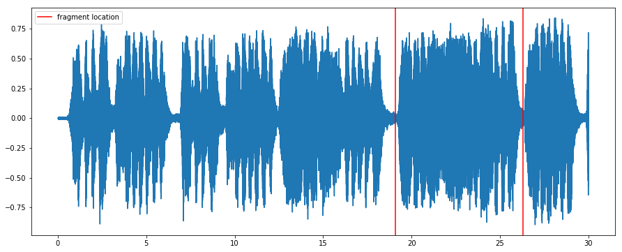
In this example, chromaprints are used to locate a segment of a larger piece after some modifications. This is an adaptation of this gist by Lukáš Lalinský. In a real world application this technique could be used, for instance, to identify songs in a DJ set stream. In this example, we will work on a short fragment of Mozart and we will try to identify the phrase among bars from the next plot.
from pylab import plot, show, figure, imshow
%matplotlib inline
import matplotlib.pyplot as plt
import numpy as np
plt.rcParams['figure.figsize'] = (15, 6) # set plot sizes to something larger than default
fs=44100
audio = es.MonoLoader(filename='../../../test/audio/recorded/mozart_c_major_30sec.wav', sampleRate=fs)() # this song is not available
time = np.linspace(0, len(audio)/float(fs), len(audio))
plot(time, audio)
# Segment limits
start = 19.1
end = 26.3
plt.axvline(x=start, color='red', label='fragment location')
plt.axvline(x=end, color='red')
plt.legend()
<matplotlib.legend.Legend at 0x7f3209427e10>
This is how the track sounds like:
IPython.display.Audio(audio, rate=44100)
In order to show the robustness of the fingerprinting algorithm, we will apply a 1st order lowpass filter tuned to 16kHz. This kind of filtering is one of the differences observed between low bitrate MP3 files and their original WAV, so the fingerprinting algorithm should be robust to this sort of alterations.
fragment = audio[int(start*fs):int(end*fs)]
fragment = es.LowPass(cutoffFrequency=16000)(fragment)
IPython.display.Audio(fragment, rate=44100)
The first step is to compute and uncompress the chromaprints of the full track and the modified segment.
import acoustid as ai
fp_full_char = es.Chromaprinter()(audio)
fp_frag_char = es.Chromaprinter()(fragment)
fp_full = ai.chromaprint.decode_fingerprint(fp_full_char)[0]
fp_frag = ai.chromaprint.decode_fingerprint(fp_frag_char)[0]
The identification proccess starts by finding the common items (or frames) of the chromaprints. At this stage, only the 20 most significative bits are used.
full_20bit = [x & (1<<20 - 1) for x in fp_full]
short_20bit = [x & (1<<20 - 1) for x in fp_frag]
common = set(full_20bit) & set(short_20bit)
For convenience, a reversed dictionary is created to access the timestamps given the 20-bit values.
def invert(arr):
"""
Make a dictionary that with the array elements as keys and
their positions positions as values.
"""
map = {}
for i, a in enumerate(arr):
map.setdefault(a, []).append(i)
return map
i_full_20bit = invert(full_20bit)
i_short_20bit = invert(short_20bit)
Now the offsets among the common items are stored:
duration = len(audio) / 44100.offsets = {}
for a in common:
for i in i_full_20bit[a]:
for j in i_short_20bit[a]:
o = i - j
offsets[o] = offsets.get(o, 0) + 1
All the detected offsets are filtered and scored. The criterium for filtering is the greatest number of common events. In this example, only the 20 top offsets are considered. The final score is computed by measuring the bit-wise distance of the 32-bit vectors given the proposed offsets.
popcnt_table_8bit = [
0,1,1,2,1,2,2,3,1,2,2,3,2,3,3,4,1,2,2,3,2,3,3,4,2,3,3,4,3,4,4,5,
1,2,2,3,2,3,3,4,2,3,3,4,3,4,4,5,2,3,3,4,3,4,4,5,3,4,4,5,4,5,5,6,
1,2,2,3,2,3,3,4,2,3,3,4,3,4,4,5,2,3,3,4,3,4,4,5,3,4,4,5,4,5,5,6,
2,3,3,4,3,4,4,5,3,4,4,5,4,5,5,6,3,4,4,5,4,5,5,6,4,5,5,6,5,6,6,7,
1,2,2,3,2,3,3,4,2,3,3,4,3,4,4,5,2,3,3,4,3,4,4,5,3,4,4,5,4,5,5,6,
2,3,3,4,3,4,4,5,3,4,4,5,4,5,5,6,3,4,4,5,4,5,5,6,4,5,5,6,5,6,6,7,
2,3,3,4,3,4,4,5,3,4,4,5,4,5,5,6,3,4,4,5,4,5,5,6,4,5,5,6,5,6,6,7,
3,4,4,5,4,5,5,6,4,5,5,6,5,6,6,7,4,5,5,6,5,6,6,7,5,6,6,7,6,7,7,8,
]
def popcnt(x):
"""
Count the number of set bits in the given 32-bit integer.
"""
return (popcnt_table_8bit[(x >> 0) & 0xFF] +
popcnt_table_8bit[(x >> 8) & 0xFF] +
popcnt_table_8bit[(x >> 16) & 0xFF] +
popcnt_table_8bit[(x >> 24) & 0xFF])
def ber(offset):
"""
Compare the short snippet against the full track at given offset.
"""
errors = 0
count = 0
for a, b in zip(fp_full[offset:], fp_frag):
errors += popcnt(a ^ b)
count += 1
return max(0.0, 1.0 - 2.0 * errors / (32.0 * count))
matches = []
for count, offset in sorted([(v, k) for k, v in offsets.items()], reverse=True)[:20]:
matches.append((ber(offset), offset))
matches.sort(reverse=True)
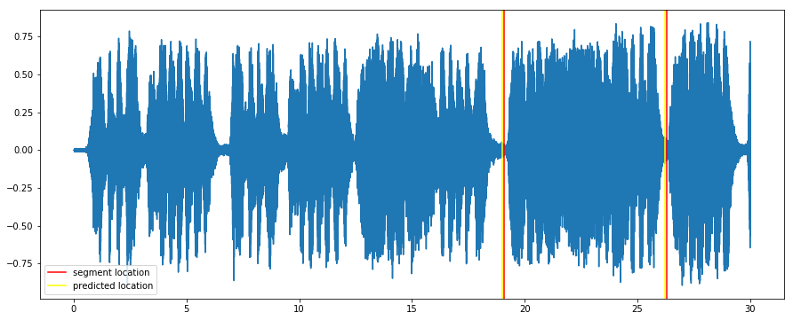
The offset with the best score is considered the optimal location of the segment.
score, offset = matches[0]
offset_secs =int(offset * 0.1238) # each fingerprint item represents 0.1238 seconds
fp_duration = len(fp_frag) * 0.1238 + 2.6476 # there is also a duration offset found empirically
print "position %d:%02d with score %f" % (offset_secs / 60, offset_secs % 60, score)
plot(time, audio)
plt.axvline(x=start, color='red', label= 'segment location')
plt.axvline(x=end, color='red')
plt.axvline(x=offset_secs, color='yellow', label='predicted location')
plt.axvline(x=offset_secs + fp_duration, color='yellow')
plt.legend()
position 0:19 with score 0.937500
<matplotlib.legend.Legend at 0x7f32093b82d0>
Cover Song Identification
Cover song identification (CSI) in MIR is a task of identifying when two musical recordings are derived from the same music composition. The cover of a song can be drastically different from the original recording. It can change key, tempo, instrumentation, musical structure or order, etc.
Essentia provides open-source implmentation of some state-of-the-art cover song identification algorithms. The following process-chain is required to use this CSI algorithms.
Tonal feature extraction. Mostly used by chroma features. Here we use HPCP.
Post-processing of the features to achieve invariance (eg. key) [3].
Cross similarity matrix computation ([1] or [2]).
Local sub-sequence alignment to compute the pairwise cover song similarity distance [1].
In this tutorial, we use HPCP, ChromaCrossSimilarity and
CoverSongSimilarity algorithms from essentia.
References:
[1]. Serra, J., Serra, X., & Andrzejak, R. G. (2009). Cross recurrence quantification for cover song identification.New Journal of Physics.
[2]. Serra, Joan, et al (2008). Chroma binary similarity and local alignment applied to cover song identification. IEEE Transactions on Audio, Speech, and Language Processing.
[3]. Serra, J., Gómez, E., & Herrera, P. (2008). Transposing chroma representations to a common key, IEEE Conference on The Use of Symbols to Represent Music and Multimedia Objects.
import essentia.standard as estd
from essentia.pytools.spectral import hpcpgram
Let’s load a query cover song, true-cover reference song and a
false-cover reference song. Here we chose a accapella cover of the
Beatles track Yesterday as our query song and it’s orginal version
by the Beatles and a cover of another Beatles track Come Together by
the Aerosmith as the reference tracks. We obtained these audio files
from the covers80 dataset
(https://labrosa.ee.columbia.edu/projects/coversongs/covers80/).
Query cover song
import IPython
IPython.display.Audio('./en_vogue+Funky_Divas+09-Yesterday.mp3')
Reference song (True cover)
IPython.display.Audio('./beatles+1+11-Yesterday.mp3')
Reference song (False cover)
IPython.display.Audio('./aerosmith+Live_Bootleg+06-Come_Together.mp3')
# query cover song
query_audio = estd.MonoLoader(filename='./en_vogue+Funky_Divas+09-Yesterday.mp3', sampleRate=32000)()
true_cover_audio = estd.MonoLoader(filename='./beatles+1+11-Yesterday.mp3', sampleRate=32000)()
# wrong match
false_cover_audio = estd.MonoLoader(filename='./aerosmith+Live_Bootleg+06-Come_Together.mp3', sampleRate=32000)()
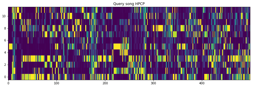
Now let’s compute Harmonic Pitch Class Profile (HPCP) chroma features of these audio signals.
query_hpcp = hpcpgram(query_audio, sampleRate=32000)
true_cover_hpcp = hpcpgram(true_cover_audio, sampleRate=32000)
false_cover_hpcp = hpcpgram(false_cover_audio, sampleRate=32000)
plotting the hpcp features
%matplotlib inline
import matplotlib.pyplot as plt
fig = plt.gcf()
fig.set_size_inches(14.5, 4.5)
plt.title("Query song HPCP")
plt.imshow(query_hpcp[:500].T, aspect='auto', origin='lower', interpolation='none')
<matplotlib.image.AxesImage at 0x7f8cd0ca2650>
Next steps are done using the essentia ChromaCrossSimilarity
function,
Stacking input features
Key invariance using Optimal Transposition Index (OTI) [3].
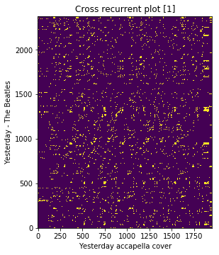
Compute binary chroma cross similarity using cross recurrent plot as described in [1] or using OTI-based chroma binary method as detailed in [3]
crp = estd.ChromaCrossSimilarity(frameStackSize=9,
frameStackStride=1,
binarizePercentile=0.095,
oti=True)
true_pair_crp = crp(query_hpcp, true_cover_hpcp)
fig = plt.gcf()
fig.set_size_inches(15.5, 5.5)
plt.title('Cross recurrent plot [1]')
plt.xlabel('Yesterday accapella cover')
plt.ylabel('Yesterday - The Beatles')
plt.imshow(true_pair_crp, origin='lower')
<matplotlib.image.AxesImage at 0x7f8cd0bee290>
Compute binary chroma cross similarity using cross recurrent plot of the non-cover pairs
crp = estd.ChromaCrossSimilarity(frameStackSize=9,
frameStackStride=1,
binarizePercentile=0.095,
oti=True)
false_pair_crp = crp(query_hpcp, false_cover_hpcp)
fig = plt.gcf()
fig.set_size_inches(15.5, 5.5)
plt.title('Cross recurrent plot [1]')
plt.xlabel('Come together cover - Aerosmith')
plt.ylabel('Yesterday - The Beatles')
plt.imshow(false_pair_crp, origin='lower')
<matplotlib.image.AxesImage at 0x7f8cd0b66ad0>
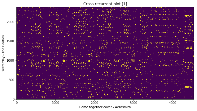
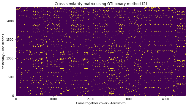
Alternatively, you can also use the OTI-based binary similarity method as explained in [2] to compute the cross similarity of two given chroma features.
csm = estd.ChromaCrossSimilarity(frameStackSize=9,
frameStackStride=1,
binarizePercentile=0.095,
oti=True,
otiBinary=True)
oti_csm = csm(query_hpcp, false_cover_hpcp)
fig = plt.gcf()
fig.set_size_inches(15.5, 5.5)
plt.title('Cross similarity matrix using OTI binary method [2]')
plt.xlabel('Come together cover - Aerosmith')
plt.ylabel('Yesterday - The Beatles')
plt.imshow(oti_csm, origin='lower')
<matplotlib.image.AxesImage at 0x7f8cd0b38e50>
Finally, we compute an asymmetric cover song similarity measure from the pre-computed binary cross simialrity matrix of cover/non-cover pairs using various contraints of smith-waterman sequence alignment algorithm (eg.
serra09orchen17).
Computing cover song similarity distance between ‘Yesterday - accapella cover’ and ‘Yesterday - The Beatles’
score_matrix, distance = estd.CoverSongSimilarity(disOnset=0.5,
disExtension=0.5,
alignmentType='serra09',
distanceType='asymmetric')(true_pair_crp)
fig = plt.gcf()
fig.set_size_inches(15.5, 5.5)
plt.title('Cover song similarity distance: %s' % distance)
plt.xlabel('Yesterday accapella cover')
plt.ylabel('Yesterday - The Beatles')
plt.imshow(score_matrix, origin='lower')
<matplotlib.image.AxesImage at 0x7f8cd0aae310>
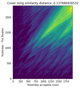
print('Cover song similarity distance: %s' % distance)
Cover song similarity distance: 0.137886926532
Computing cover song similarity distance between
Yesterday - accapella cover and
Come Together cover - The Aerosmith.
score_matrix, distance = estd.CoverSongSimilarity(disOnset=0.5,
disExtension=0.5,
alignmentType='serra09',
distanceType='asymmetric')(false_pair_crp)
fig = plt.gcf()
fig.set_size_inches(15.5, 5.5)
plt.title('Cover song similarity distance: %s' % distance)
plt.xlabel('Yesterday accapella cover')
plt.ylabel('Come together cover - Aerosmith')
plt.imshow(score_matrix, origin='lower')
<matplotlib.image.AxesImage at 0x7f8cd0a1b390>
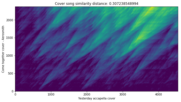
print('Cover song similarity distance: %s' % distance)
Cover song similarity distance: 0.307238548994
Voila! We can see that the cover similarity distance is quite low for the actual cover song pairs as expected.
Inference with TensorFlow models
Essentia supports inference with TensorFlow models for a variety of MIR tasks.
The following examples complement our blog posts and publications [1, 2] covering this topic.
Visit our blog for more details about the framework and find the models available at our website.
References:
[1] Alonso-Jiménez, P., Bogdanov, D., Pons, J., & Serra, X. Tensorflow Audio Models in Essentia. IEEE International Conference on Acoustics, Speech and Signal Processing (ICASSP’20) (pp. 266-270). 2020.
[2] Alonso-Jiménez, P., Bogdanov, D., & Serra, X. Deep embeddings with Essentia models. International Conference on Music Information Retrieval (ISMIR’20), LBD. 2020.
Auto-tagging
In this example, we predict musical tags for a music track using the
MusiCNN model and plot the resulting tag activations over time
(tag-gram).
The first step is to download the model and the metadata file attached to it from our website.
!curl -SLO https://essentia.upf.edu/models/autotagging/msd/msd-musicnn-1.pb
!curl -SLO https://essentia.upf.edu/models/autotagging/msd/msd-musicnn-1.json
% Total % Received % Xferd Average Speed Time Time Time Current
Dload Upload Total Spent Left Speed
100 3123k 100 3123k 0 0 23.6M 0 --:--:-- --:--:-- --:--:-- 23.6M
% Total % Received % Xferd Average Speed Time Time Time Current
Dload Upload Total Spent Left Speed
100 2100 100 2100 0 0 43750 0 --:--:-- --:--:-- --:--:-- 44680
The metadata file contains information about the model such as the name of the most relevant layers, the classes it can predict, the data used for training, or evaluation metrics when available.
import json
musicnn_metadata = json.load(open('msd-musicnn-1.json', 'r'))
for k, v in musicnn_metadata.items():
print('{}: {}'.format(k , v))
name: MSD MusiCNN type: auto-tagging link: https://essentia.upf.edu/models/autotagging/msd/msd-musicnn-1.pb version: 1 description: prediction of the top-50 tags in the dataset author: Pablo Alonso email: pablo.alonso@upf.edu release_date: 2020-03-31 framework: tensorflow framework_version: 1.15.0 classes: ['rock', 'pop', 'alternative', 'indie', 'electronic', 'female vocalists', 'dance', '00s', 'alternative rock', 'jazz', 'beautiful', 'metal', 'chillout', 'male vocalists', 'classic rock', 'soul', 'indie rock', 'Mellow', 'electronica', '80s', 'folk', '90s', 'chill', 'instrumental', 'punk', 'oldies', 'blues', 'hard rock', 'ambient', 'acoustic', 'experimental', 'female vocalist', 'guitar', 'Hip-Hop', '70s', 'party', 'country', 'easy listening', 'sexy', 'catchy', 'funk', 'electro', 'heavy metal', 'Progressive rock', '60s', 'rnb', 'indie pop', 'sad', 'House', 'happy'] model_types: ['frozen_model'] dataset: {'name': 'The Millon Song Dataset', 'citation': 'http://millionsongdataset.com/', 'size': '200k up to two minutes audio previews', 'metrics': {'ROC-AUC': 0.88, 'PR-AUC': 0.29}} schema: {'inputs': [{'name': 'model/Placeholder', 'type': 'float', 'shape': [187, 96]}], 'outputs': [{'name': 'model/Sigmoid', 'type': 'float', 'shape': [1, 50], 'op': 'Sigmoid'}, {'name': 'model/dense_1/BiasAdd', 'type': 'float', 'shape': [1, 50], 'op': 'fully connected', 'description': 'logits'}, {'name': 'model/dense/BiasAdd', 'type': 'float', 'shape': [1, 200], 'op': 'fully connected', 'description': 'embeddings'}]} citation: @article{alonso2020tensorflow, title={TensorFlow Audio Models in Essentia}, author={Alonso-Jim{'e}nez, Pablo and Bogdanov, Dmitry and Pons, Jordi and Serra, Xavier}, journal={ICASSP 2020}, year={2020} }
We have specific algorithms to perform predictions by each model.
TensorflowPredictMusiCNN
is tailored to operate with MusiCNN and MusiCNN-based models as
we will see later on.
You can go to the reference page and read the algorithm’s documentation to check the algorithm input requirements.
TensorflowPredictMusiCNN expects audio with a sample rate of 16kHz
as input. We can obtain it using MonoLoader algorithm modifying its
sampleRate parameter accordingly.
Let’s make some predictions now!
sr = 16000
audio = es.MonoLoader(filename='../../../test/audio/recorded/techno_loop.wav', sampleRate=sr)()
musicnn_preds = es.TensorflowPredictMusiCNN(graphFilename='msd-musicnn-1.pb')(audio)
Finally we can get the classes from the metadata to label the \(y\) axis of the tag-gram.
classes = musicnn_metadata['classes']
plt.matshow(musicnn_preds.T)
plt.title('taggram')
plt.yticks(np.arange(len(classes)), classes)
plt.gca().xaxis.set_ticks_position('bottom')
plt.show()
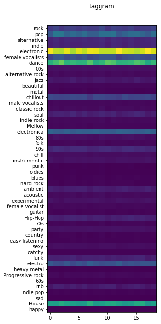
We can see that the model produced 19 predictions (\(x\) axis). This
is because by default MusiCNN operates on 3-second patches with an
overlap of 1.5 seconds and our example lasts 30 seconds.
Transfer learning classifiers
In this example, we are learning how to use our transfer learning classifiers.
These classifiers were trained on top of bigger models such as
MusiCNN to leverage the audio representations learned on larger
amounts of data. For clarity, the classifiers are named following this
convention: <targer-task>-<source-task>-<version>. So
danceability-musicnn-msd-2.pb is a danceability classifier
trained on top of the musicnn-msd model and it is the release
version number 2.
The algorithm to use is determined by the source-task, so again we
should use TensorFlowPredictMusiCNN.
!curl -SLO https://essentia.upf.edu/models/classifiers/danceability/danceability-musicnn-msd-2.pb
!curl -SLO https://essentia.upf.edu/models/classifiers/danceability/danceability-musicnn-msd-2.json
% Total % Received % Xferd Average Speed Time Time Time Current
Dload Upload Total Spent Left Speed
100 3163k 100 3163k 0 0 25.5M 0 --:--:-- --:--:-- --:--:-- 25.7M
% Total % Received % Xferd Average Speed Time Time Time Current
Dload Upload Total Spent Left Speed
100 1736 100 1736 0 0 7890 0 --:--:-- --:--:-- --:--:-- 7855
danceability_preds = es.TensorflowPredictMusiCNN(graphFilename='danceability-musicnn-msd-2.pb')(audio)
danceability_metadata = json.load(open('danceability-musicnn-msd-2.json', 'r'))['classes']
# Average predictions over the time axis
danceability_preds = np.mean(danceability_preds, axis=0)
print('{}: {}%'.format(danceability_metadata[0] , danceability_preds[0] * 100))
danceable: 100.0%
Tempo estimation
We provide tempo estimation through the TempoCNN models. In this
case, we do not need any metadata information as this model is not
returning class probabilities but the most likely BPM value directly.
!curl -SLO https://essentia.upf.edu/models/tempo/tempocnn/deeptemp-k16-3.pb
% Total % Received % Xferd Average Speed Time Time Time Current
Dload Upload Total Spent Left Speed
100 1289k 100 1289k 0 0 14.8M 0 --:--:-- --:--:-- --:--:-- 14.8M
sr = 11025
audio_11khz = es.MonoLoader(filename='../../../test/audio/recorded/techno_loop.wav', sampleRate=sr)()
global_bpm, local_bpm, local_probs = es.TempoCNN(graphFilename='deeptemp-k16-3.pb')(audio_11khz)
print('song BPM: {}'.format(global_bpm))
song BPM: 125.0
We can plot a slice of the waveform on top of a grid with the estimated tempo to get visual verification
duration = 5 # seconds
audio_slice = audio_11khz[:sr * duration]
plt.plot(audio_slice)
markers = np.arange(0, len(audio_slice), sr / (global_bpm / 60))
for marker in markers:
plt.axvline(x=marker, color='red')
plt.title("Audio waveform on top of a tempo grid")
Text(0.5, 1.0, 'Audio waveform on top of a tempo grid')
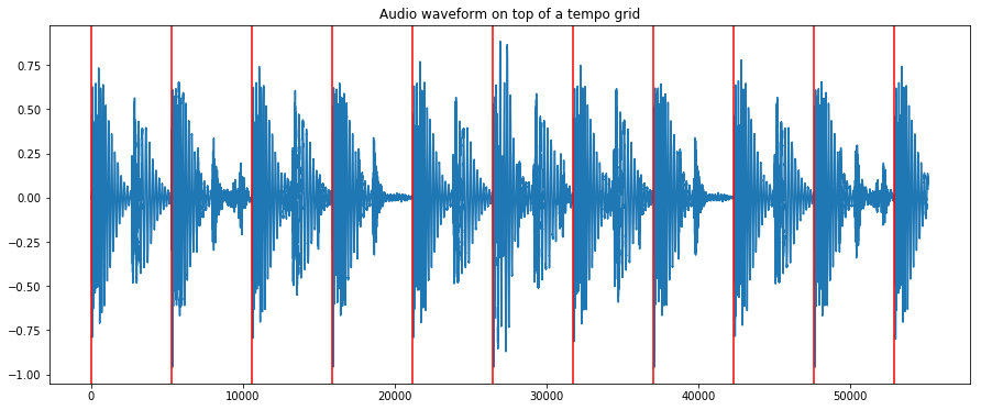
TempoCNN operates on audio slices of 12 seconds with an overlap of 6
seconds by default. Additionally, the algorithm outputs the local
estimations along with their probabilities. The global value is computed
by majority voting by default. However, this method is only recommended
when a constant tempo can be assumed.
print('local BPM: {}'.format(local_bpm))
print('local probabilities: {}'.format(local_probs))
local BPM: [125. 125. 125. 125.]
local probabilities: [0.9679363 0.96005017 0.9681525 0.96270114]
You can notice how the model gives very high probabilities to all the estimations. This is because we chose an example with a very tight beat.
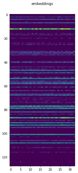
Embedding extraction
In the next example, we are computing embeddings with the VGGish
model.
!curl -SLO https://essentia.upf.edu/models/feature-extractors/vggish/audioset-vggish-3.pb
% Total % Received % Xferd Average Speed Time Time Time Current
Dload Upload Total Spent Left Speed
100 275M 100 275M 0 0 34.8M 0 0:00:07 0:00:07 --:--:-- 34.9M
sr = 16000
audio = es.MonoLoader(filename='../../../test/audio/recorded/techno_loop.wav', sampleRate=sr)()
vggish_preds = es.TensorflowPredictVGGish(graphFilename='audioset-vggish-3.pb',
output='model/vggish/embeddings')(audio)
plt.matshow(vggish_preds.T, aspect=.6)
plt.title('embeddings')
plt.gca().xaxis.set_ticks_position('bottom')
Extracting embeddings from other models
In every TensorFlow prediction algorithm, you can choose the layer of the model to retrieve. One application of this is to use any model as an embedding extractor.
For some models, we even suggest a layer that could be used as
embeddings. Let’s see the information about the outputs for the
MusiCNN model we loaded before.
print('Model outputs:\n')
for output in musicnn_metadata['schema']['outputs']:
for k, v in output.items():
print('{}: {}'.format(k , v))
print()
Model outputs:
name: model/Sigmoid
type: float
shape: [1, 50]
op: Sigmoid
name: model/dense_1/BiasAdd
type: float
shape: [1, 50]
op: fully connected
description: logits
name: model/dense/BiasAdd
type: float
shape: [1, 200]
op: fully connected
description: embeddings
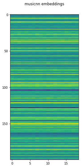
From this we learn that the output of the penultimate dense layer is
proposed as embeddings. We can extract it by setting the output
parameter.
musicnn_embs = es.TensorflowPredictMusiCNN(graphFilename='msd-musicnn-1.pb',
output='model/dense/BiasAdd')(audio)
plt.matshow(musicnn_embs.T, aspect=.2)
plt.title('musicnn embeddings')
plt.gca().xaxis.set_ticks_position('bottom')
