Music auto-tagging, classification, and embedding extraction¶

Setup¶

First of all, notice that the default Essentia’s pip package does not include TensorFlow support. Currently, this is only available through pip for Linux with Python >=3.5 and <=3.7.

!pip install -q essentia-tensorflow

Alternatively, you can follow the instructions in this blog post to build Essentia with TensorFlow support. This approach also works in Mac, for Python >=3.8 or with TensorFlow >=2.0.

After this step, we can import the required packages.

import json

from essentia.standard import MonoLoader, TensorflowPredictMusiCNN, TensorflowPredictVGGish
import numpy as np
import matplotlib.pyplot as plt

The Essentia models’ site contains models for diverse purposes. Each model comes with a .json metadata file with information such as the classes it can predict, the metrics achieved on training, or the model’s version.

Let’s download the MusiCNN auto-tagging model trained on the Million Song Dataset.

!wget -q https://essentia.upf.edu/models/autotagging/msd/msd-musicnn-1.pb
!wget -q https://essentia.upf.edu/models/autotagging/msd/msd-musicnn-1.json

We can open the metadata file and check all the available keys.

with open('msd-musicnn-1.json', 'r') as json_file:
    metadata = json.load(json_file)

print(metadata.keys())

dict_keys(['name', 'type', 'link', 'version', 'description', 'author', 'email', 'release_date', 'framework', 'framework_version', 'classes', 'model_types', 'dataset', 'schema', 'citation'])

Finally, we load an audio file to use as an example.

audio_file = '../../../test/audio/recorded/techno_loop.wav'
audio = MonoLoader(sampleRate=16000, filename=audio_file)()

Auto-tagging¶

Now we have all the ingredients to perform auto-tagging with MusiCNN. TensorflowPredictMusiCNN is our dedicated algorithm to make predictions with models expecting MusiCNN’s mel-spectrogram signature. We have to configure the graphFilename parameter with the path to the model and feed the algorithm with audio sampled at 16kHz. The output is a two-dimensional matrix [time, activations].

activations = TensorflowPredictMusiCNN(graphFilename='msd-musicnn-1.pb')(audio)

Finally, we use matplotlib to plot the activations.

ig, ax = plt.subplots(1, 1, figsize=(10, 10))
ax.matshow(activations.T, aspect='auto')

ax.set_yticks(range(len(metadata['classes'])))
ax.set_yticklabels(metadata['classes'])
ax.set_xlabel('patch number')
ax.xaxis.set_ticks_position('bottom')
plt.title('Tag activations')
plt.show()

Classification with the transfer learning classifiers¶

Essentia is shipped with a collection of single-label classifiers based on transfer learning that rely on our auto-tagging models or other deep embedding extractors. You can read our blog post for a complete list of the available classifiers.

In this example, we use the danceability classifier based on the VGGish model.

!wget -q https://essentia.upf.edu/models/classifiers/danceability/danceability-vggish-audioset-1.pb
!wget -q https://essentia.upf.edu/models/classifiers/danceability/danceability-vggish-audioset-1.json

We use the TensorflowPredictVGGish algorithm because it generates the required mel-spectrogram signature for this case, but if we wanted to use the danceability classifier based on MusiCNN we should use TensorflowPredictMusiCNN again.

with open('danceability-vggish-audioset-1.json', 'r') as json_file:
    metadata = json.load(json_file)

activations = TensorflowPredictVGGish(graphFilename='danceability-vggish-audioset-1.pb')(audio)

Finally, we can compute the global accuracy as the mean of the activations along the temporal axis.

for label, probability in zip(metadata['classes'], activations.mean(axis=0)):
    print(f'{label}: {100 * probability:.1f}%')

danceable: 99.8%
not_danceable: 0.2%

Embedding extraction¶

A usual transfer learning approach consists of extracting low-dimensional feature maps from one of the last layers of a pre-trained model as embeddings for a new downstream task. The metadata includes a field schema with the names of the most relevent layers of each model, including layers that are suitable for embedding extraction.

with open('msd-musicnn-1.json', 'r') as json_file:
    metadata = json.load(json_file)

print(metadata['schema'])

{'inputs': [{'name': 'model/Placeholder', 'type': 'float', 'shape': [187, 96]}], 'outputs': [{'name': 'model/Sigmoid', 'type': 'float', 'shape': [1, 50], 'op': 'Sigmoid'}, {'name': 'model/dense_1/BiasAdd', 'type': 'float', 'shape': [1, 50], 'op': 'fully connected', 'description': 'logits'}, {'name': 'model/dense/BiasAdd', 'type': 'float', 'shape': [1, 200], 'op': 'fully connected', 'description': 'embeddings'}]}

From this, we see that model/dense_1/BiasAdd is the recommended layer for embeddings. Additionally, an external tool such as Netron can be used to inspect the model and get the information about the whole architecture.

TensorflowPredictMusiCNN offers an output parameter that can be configured to select the layer of the model to retrieve.

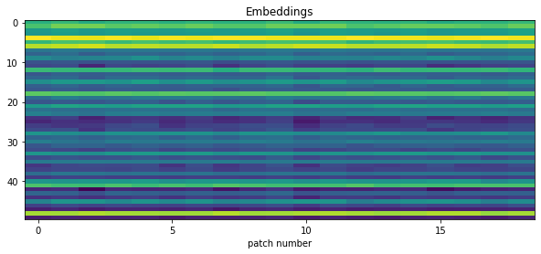
embeddings = TensorflowPredictMusiCNN(graphFilename='msd-musicnn-1.pb', output='model/dense_1/BiasAdd')(audio)

ig, ax = plt.subplots(1, 1, figsize=(10, 4))
ax.matshow(embeddings.T, aspect='auto')
ax.xaxis.set_ticks_position('bottom')
ax.set_xlabel('patch number')
plt.title('Embeddings')
plt.show()