NSGConstantQ Examples
This notebook provides practical examples of using the NSGConstantQ algorithm.
import numpy as np
import matplotlib.pyplot as plt
from essentia import Pool
from essentia import run
import essentia.streaming as streaming
import essentia.standard as standard

%matplotlib inline
plt.rcParams['figure.figsize'] = (8.0, 6.0)
eps = np.finfo(np.float64).eps
Configuring the algorithm
In this example the algorithm is configured to analyse a fragment of
male singing voice. The frequency range we want to analyze is set
accordingly. The minimum frequency is set to match the freqeuncy of a
note (C2 in this case). The binsPerOctave is set to a miltiple of 12
so that the frequency channels (bands) we want to compute match
subdivisions of an equal tempered scale (in our case, 4 bins per
semitone).
rasterize controls the interpolation on the frequency channels. When
set to ‘full’, frequency channels will have the same lengths. The ‘full’
interpolation is mandatory if one wants to stream frames in the
streaming mode.
If one wants to perform transformations in the constant-Q domain and then go back to the time domain, both direct and inverse algorithms (NSGConstantQ and NSGIConstantQ) should be configured with exactly the same parameters. The easiest way to do this is to use a dictionary for configuring both algorithms’ parameters.
kwargs = {
'inputSize': 4096,
'minFrequency': 65.41,
'maxFrequency': 6000,
'binsPerOctave': 48,
'sampleRate': 44100,
'rasterize': 'full',
'phaseMode': 'global',
'gamma': 0,
'normalize': 'none',
'window': 'hannnsgcq',
}
Standard mode
Standard mode is very simple to use. In this example we transform a
singing voice into the Gabor domain and then compute back its time
representation. It is important to configure both algorithms with the
same parameters. It is especially important to set inputSize so that
the inverse algorithm is able to reconstruct the input signal.
x = standard.MonoLoader(filename = '../../../test/audio/recorded/vignesh.wav')()[:-1]
# Remove the last sample to make the signal even

kwargs['inputSize'] = len(x)

CQStand = standard.NSGConstantQ(**kwargs)
CQIStand = standard.NSGIConstantQ(**kwargs)

constantq, dcchannel, nfchannel = CQStand(x)
y = CQIStand(constantq, dcchannel, nfchannel)
NSGConstantQ outputs three vectors. The first one (constantq) is the
actual transform and it is a complex time-frequency representation of
the input audio. Depending on the rasterize parameter it will behave
differently:
‘none’: each frequency channel will have the minimum length needed give full frequency support to its bandwidth. The
constantqoutput is a list of lists.‘piecewise’: adds some interpolation to make the length of each channel a power of 2 in order to perform optimized FFTs.
‘full’: interpolates the channels so that they all have the same length and the
constantqoutput is a square matrix (i.e., a 2D complex numpy matrix). This may be the easiest way to manipulate the data afterwards.
The other two outputs (dcchannel and mfchannel) are only
important in order to compute the inverse transform.
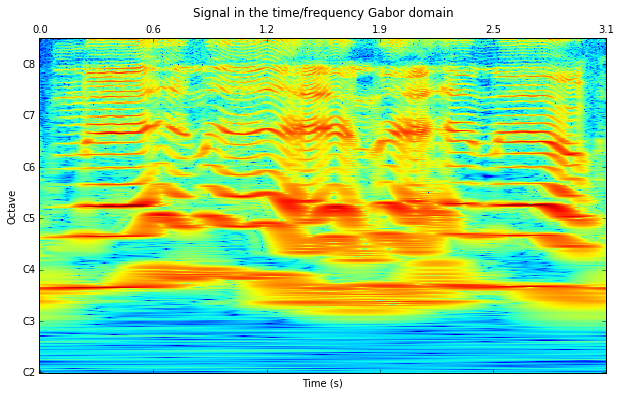
Constant-Q spectrogram
Finally, let’s see how our transform looks like. As the constantq
variable is a complex 2D matrix, we compute its absolute values and then
apply log-transform to obtain the log-spectrogram.
# Time labeling
ticksTime = np.linspace(0, len(constantq.T), 6)
secs = np.around(ticksTime * kwargs['inputSize'] /  (kwargs['sampleRate'] * len(constantq.T) ) , decimals=1)
# Octave labeling
ticksFreq = np.arange(0,len(constantq),kwargs['binsPerOctave'])
notes =  ['C%i' %f for f in range(2, len(ticksFreq) +2, 1) ]

plt.matshow(np.log(np.abs(constantq)),origin='lower')
plt.yticks(ticksFreq, notes)
plt.xticks(ticksTime, secs)
plt.ylabel('Octave')
plt.xlabel('Time (s)')
plt.title('Signal in the time/frequency Gabor domain')
plt.show()
Reconstructed signal
plt.plot(y)
plt.title('Re-Synthetised signal')
plt.show()

SNR = np.mean(20*np.log10(np.abs(x[100:-100])/np.abs(x[100:-100]-y[100:-100] + eps) + eps))
print 'Synthesis SNR: %.3f dB' %SNR
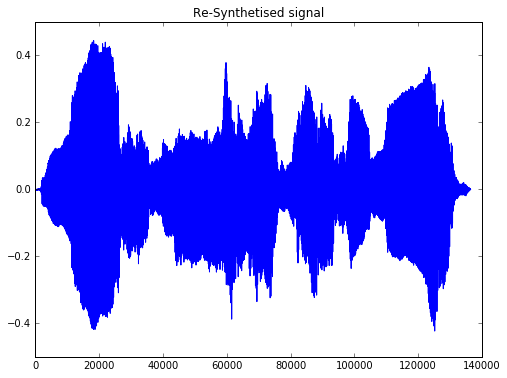
Synthesis SNR: 137.906 dB
Last time this script was executed, the maximun difference between the original and the sinthetized signal was 1.7883e-07. Provided that Essentia analysis is performed using 32-byte floats (eps = 1.192-07), this lets the systhesis error in the range of the numerical error. Thus, it can be considered a theoretically perfect reconstruction.
Streaming mode
Now let’s reimplement the same example in the streaming mode. Here we will also perform a frame-wise analysis, suitable for a real-time implementation.
First, let’s instantiate the algorithms needed for the frame-wise
analysis. We are using CartesianToPolar to save magnitude and phase
values to a Pool (as it is currently not possible to save complex arrays
to Essentia’s pools).
The length of the frames chosen for the analysis is 8192 with a hop size of 4096 using triangular windows. This framework makes it possible to obtain a perfect reconstruction but it is not the only one. Some other windows and sizes combinations are showed at the end of this notebook.
kwargs['inputSize'] = 4096 * 2

CQAlgo = streaming.NSGConstantQStreaming(**kwargs)
ICQAlgo = streaming.NSGIConstantQ(**kwargs)
loader = streaming.MonoLoader(filename='../../../test/audio/recorded/vignesh.wav')
w = streaming.Windowing(type='triangular',normalized=False, zeroPhase=False)
frameCutter = streaming.FrameCutter(frameSize=kwargs['inputSize'], hopSize=kwargs['inputSize']/2)

CQc2p = streaming.CartesianToPolar()
DCc2p = streaming.CartesianToPolar()
NFc2p = streaming.CartesianToPolar()

pool = Pool()
Let’s run the network and save the data to the pool. The actual
transform is sent through the constantq source. It is the only
output needed for the analysis purposes. However, if the goal is to
modify it and go back to the time domain, two extra outputs, containing
the DC and the Nyquist channels, are required. These outputs contain the
information below and above the analysis range and are required for the
reconstruction of the signal. Additionally, a vector called
‘framestamps’ is returned in order to facilitate the reconstruction of
the data.
´constantq´ shape is ( timestamps , number of channels )
´constantqdc´ shape is ( framestamps , length of th DC channel )
´constantqnf´ shape is ( framestamps , length of th Nyquist channel )
´framestamps´ shape is ( framestamps )
Framewise vectors are returned once per call. Timewise vectores are returned more than one token per call and their number depends on the configuration parameters. Using these matrices may be confusing, as the original algorithm (on which our implementation is based) was not intended for real-time processing.
# Conecting the algorithms
loader.audio >> frameCutter.signal

frameCutter.frame >> w.frame >> CQAlgo.frame

CQAlgo.constantq >> CQc2p.complex
CQAlgo.constantqdc >> DCc2p.complex
CQAlgo.constantqnf >> NFc2p.complex
CQAlgo.framestamps >> (pool, 'frameStamps')

CQc2p.magnitude >> (pool, 'CQmag')
CQc2p.phase >> (pool, 'CQphas')

DCc2p.magnitude >> (pool, 'DCmag')
DCc2p.phase >> (pool, 'DCphas')

NFc2p.magnitude >> (pool, 'NFmag')
NFc2p.phase >> (pool, 'NFphas')

run(loader)
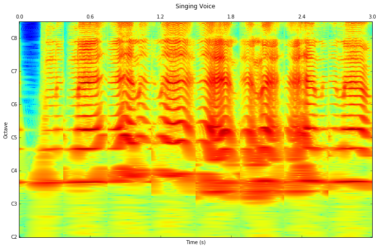
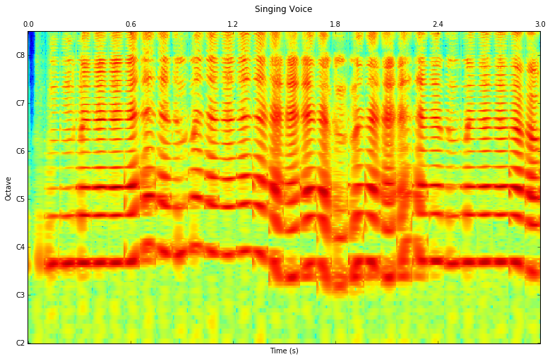
Plotting the transform
# Time labeling
ticksTime = np.linspace(0, len(pool['CQmag']), 6)
secs = np.around(ticksTime * kwargs['inputSize'] / (2 * kwargs['sampleRate'] * pool['frameStamps'][1] ), decimals=1)

# Octave labeling
ticksFreq = np.arange(0,len(pool['CQmag'].T),kwargs['binsPerOctave'])
notes =  ['C%i' %f for f in range(2, len(ticksFreq) +2, 1) ]


f, ax = plt.subplots(1, figsize = (13,10))
ax.matshow(np.log(pool['CQmag'].T),origin='lower', aspect=2)
plt.yticks(ticksFreq, notes)
plt.xticks(ticksTime, secs)
plt.ylabel('Octave')
plt.xlabel('Time (s)')
plt.title('Singing Voice')
plt.show()

# Using the same arguments for inverse transformation as for the analysis
ICQAlgo = standard.NSGIConstantQ(**kwargs)

# Loop to store the frames. DC and Nyquist channels are just tranformed into cartesian coordinates again.
recFrame = []
for i in range(len(pool['DCmag'])-1):
    invDC = standard.PolarToCartesian()(pool['DCmag'][i], pool['DCphas'][i])
    invNF = standard.PolarToCartesian()(pool['NFmag'][i], pool['NFphas'][i])

    # Concatenate CQ frames. Here it is done using the 'frameStamp' vector.
    invCQ = []
    for j in range(pool['frameStamps'][i], pool['frameStamps'][i+1],1):
        invCQ.append(standard.PolarToCartesian()(pool['CQmag'][j], pool['CQphas'][j]))

    # A trick to transpose a list of lists.
    invCQlist = [list(x) for x in zip(*invCQ)]

    # The actual inverse transform.
    recFrame.append(ICQAlgo(invCQlist, invDC, invNF))


# Overlaped addition of the input
frameSize = kwargs['inputSize']

y = recFrame[0]

invWindow = standard.Windowing(type='triangular',normalized=False, zeroPhase=False)(standard.essentia.array(np.ones(frameSize)))


for i in range(1,len(recFrame)):
    y = np.hstack([y,np.zeros(frameSize/2)])
    y[-frameSize:] = y[-frameSize:] + recFrame[i]

y = y[frameSize/2:]
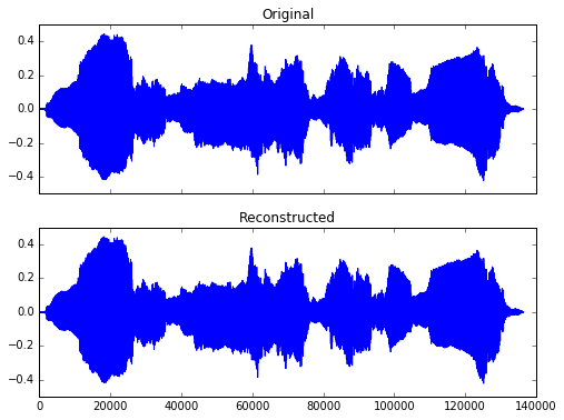
Reconstruction from Pool in standard mode
This is ugliest cell of this notebook! It shows how to return to the time domain from the constant-Q transform data stored in the pool using the standard mode again.
We can compare the original and the synthetised signals and compute the SNR of the algorithm
x = standard.MonoLoader(filename = '../../../test/audio/recorded/vignesh.wav')()
xtest = x[:len(y)]

SNR = np.mean(20*np.log10(np.abs(xtest)/np.abs(xtest-y + eps) + eps))
print 'SNR: %.3f dB' %SNR

_, ax = plt.subplots(2, sharex=True)
ax[0].plot(xtest)
ax[0].set_title('Original')
ax[1].plot(y)
ax[1].set_title('Reconstructed')
plt.show()
SNR: 137.799 dB
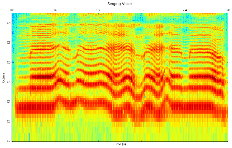
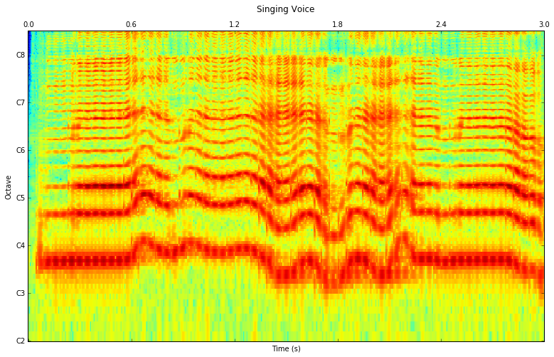
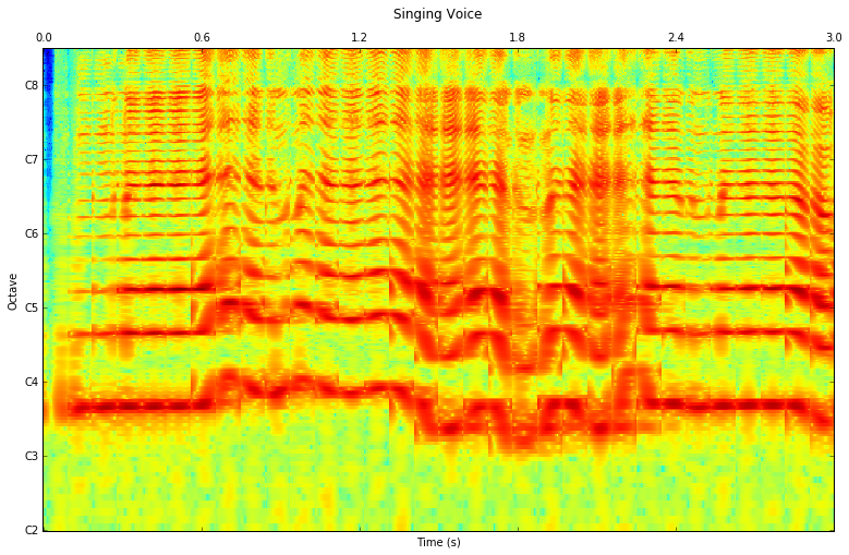
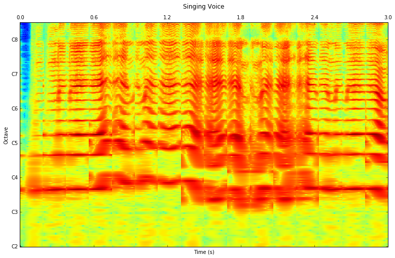
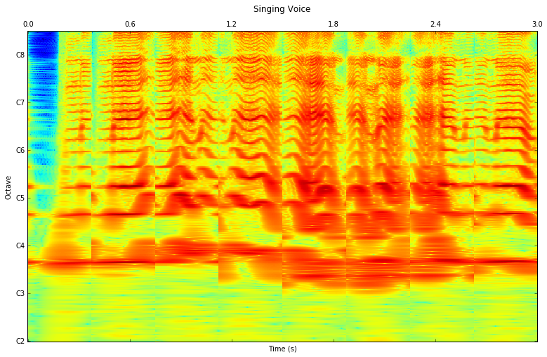
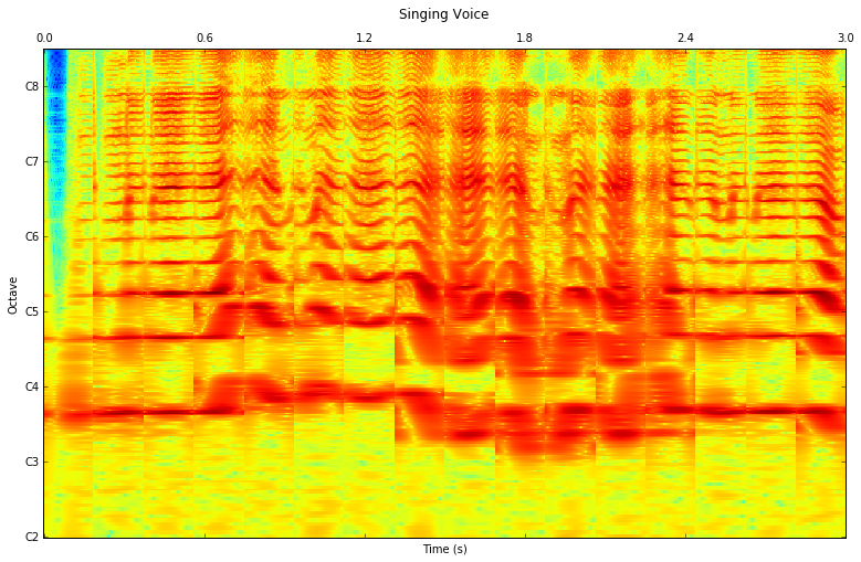
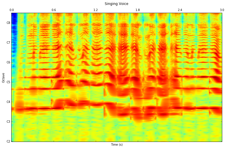
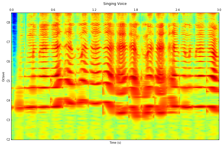
The effect of frame size and window type on constant-q spectrogram in the streaming mode
def compute_cq(kwargs):
    w = streaming.Windowing(type=kwargs['frameWindow'], normalized=False, zeroPhase=False)
    del kwargs['frameWindow']

    CQAlgo = streaming.NSGConstantQStreaming(**kwargs)
    loader = streaming.MonoLoader(filename='../../../test/audio/recorded/vignesh.wav')
    frameCutter = streaming.FrameCutter(frameSize=kwargs['inputSize'], hopSize=kwargs['inputSize']/2)

    CQc2p = streaming.CartesianToPolar()
    DCc2p = streaming.CartesianToPolar()
    NFc2p = streaming.CartesianToPolar()

    pool = Pool()

    # Conecting the algorithms
    loader.audio >> frameCutter.signal
    frameCutter.frame >> w.frame >> CQAlgo.frame

    CQAlgo.constantq >> CQc2p.complex
    CQAlgo.constantqdc >> DCc2p.complex
    CQAlgo.constantqnf >> NFc2p.complex
    CQAlgo.framestamps >> (pool, 'frameStamps')

    CQc2p.magnitude >> (pool, 'CQmag')
    CQc2p.phase >> (pool, 'CQphas')

    DCc2p.magnitude >> (pool, 'DCmag')
    DCc2p.phase >> (pool, 'DCphas')

    NFc2p.magnitude >> (pool, 'NFmag')
    NFc2p.phase >> (pool, 'NFphas')

    run(loader)

    # Plot results
    # Time labeling
    ticksTime = np.linspace(0, len(pool['CQmag']), 6)
    secs = np.around(ticksTime * kwargs['inputSize'] / (2 * kwargs['sampleRate'] * pool['frameStamps'][1] ), decimals=1)

    # Octave labeling
    ticksFreq = np.arange(0,len(pool['CQmag'].T),kwargs['binsPerOctave'])
    notes =  ['C%i' %f for f in range(2, len(ticksFreq) +2, 1) ]

    f, ax = plt.subplots(1, figsize = (13,10))
    ax.matshow(np.log(pool['CQmag'].T),origin='lower', aspect=2)
    plt.yticks(ticksFreq, notes)
    plt.xticks(ticksTime, secs)
    plt.ylabel('Octave')
    plt.xlabel('Time (s)')
    plt.title('Singing Voice')
    plt.show()


framesize = [2048, 2048*2, 2048*4, 2048*8, 2048*16]
frame_window = ["triangular", "hamming", "hann", "blackmanharris62"]

for fw in frame_window:
    for fs in framesize:
        print "Frame window:", fw
        print "Frame size:", fs
        kwargs['inputSize'] = fs
        kwargs['frameWindow'] = fw
        compute_cq(kwargs)
Frame window: triangular
Frame size: 2048
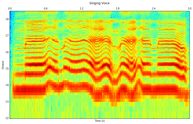
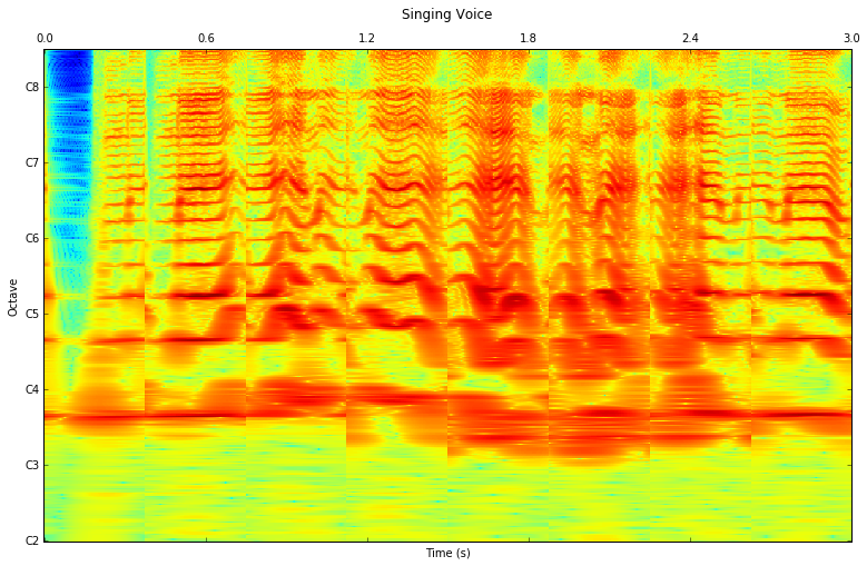
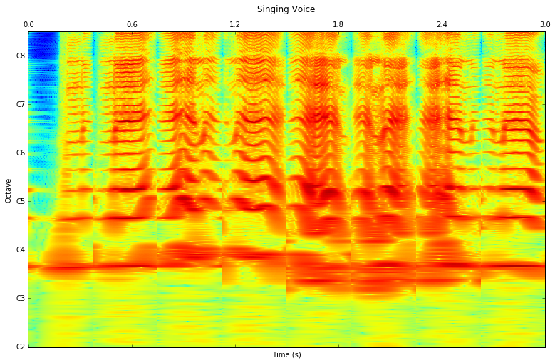
Frame window: triangular
Frame size: 4096
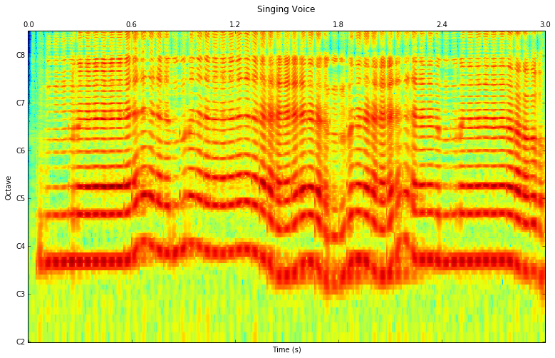
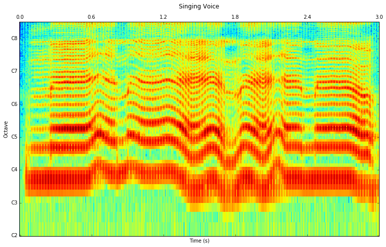
Frame window: triangular
Frame size: 8192
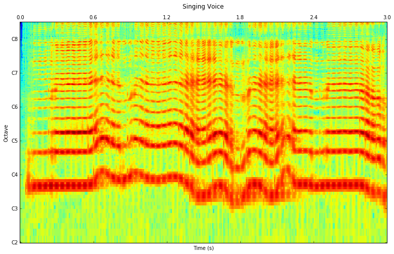
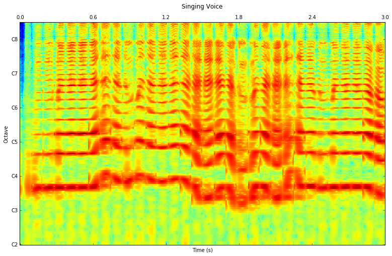
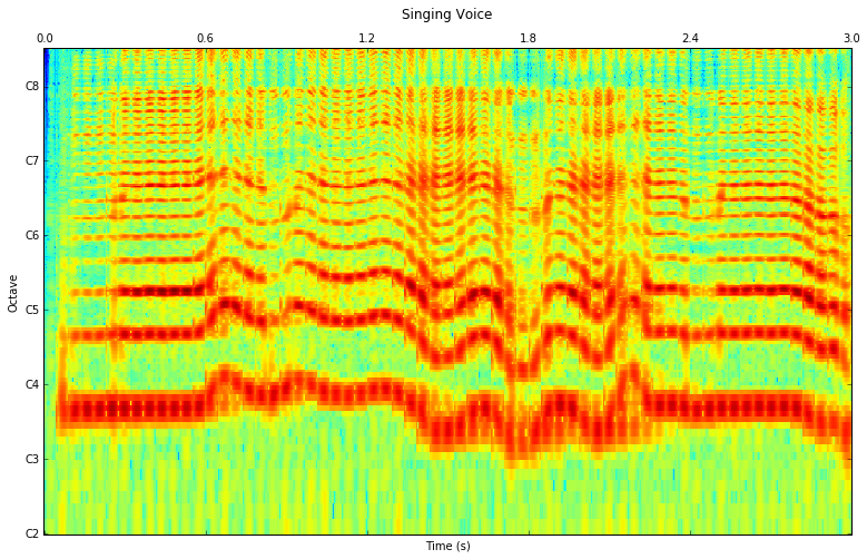
Frame window: triangular
Frame size: 16384
Frame window: triangular
Frame size: 32768
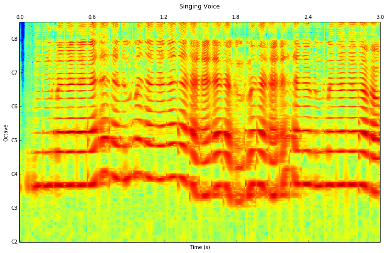
Frame window: hamming
Frame size: 2048
Frame window: hamming
Frame size: 4096
Frame window: hamming
Frame size: 8192
Frame window: hamming
Frame size: 16384
Frame window: hamming
Frame size: 32768
Frame window: hann
Frame size: 2048

Frame window: hann
Frame size: 4096
Frame window: hann
Frame size: 8192
Frame window: hann
Frame size: 16384
Frame window: hann
Frame size: 32768
Frame window: blackmanharris62
Frame size: 2048
Frame window: blackmanharris62
Frame size: 4096
Frame window: blackmanharris62
Frame size: 8192
Frame window: blackmanharris62
Frame size: 16384
Frame window: blackmanharris62
Frame size: 32768